

44
5 Analysis
10
2
10
3
10
4
(rad/sec)
0
0.2
0.4
0.6
0.8
1
S ( ) (
0
2
/Hz)
10
-4
0
1
2
S
B
z
( ) (T
2
/Hz)
10
-22
1.2
1.23
1.26
1.29
1.32
1.35
1.4
1.45
1.5
1.55
1.6
1.7
1.8
2
2.25
2.5
3
3.5
4
Temperature (K)
1.6
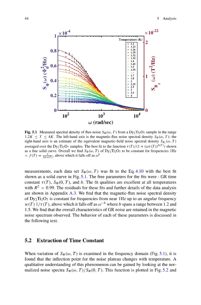
Fig. 5.1 Measured spectral density of flux-noise S (ω, T ) from a Dy 2 Ti 2 O 7 sample in the range
1.2K ≤ T ≤ 4K. The left-hand axis is the magnetic-flux noise spectral density S (ω, T ); the
right-hand axis is an estimate of the equivalent magnetic-field noise spectral density S Bz (ω, T )
averaged over the Dy 2 Ti 2 O 7 samples. The best fit to the function τ (T )/(1 + (ωτ (T )) b(T ) ) shown
as a fine solid curve. Overall we find S (ω, T ) of Dy 2 Ti 2 O 7 to be constant for frequencies 1Hz
< f (T ) =
1
2πτ (T ) , above which it falls off as ω b
measurements, each data set S (ω, T ) was fit to the Eq. 4.10 with the best fit
shown as a solid curve in Fig. 5.1. The free parameters for the fits were : GR time
constant τ (T ), S (0, T ), and b. The fit qualities are excellent at all temperatures
with R 2 > 0.99. The residuals for these fits and further details of the data analysis
are shown in Appendix A.3. We find that the magnetic-flux noise spectral density
of Dy 2 Ti 2 O 7 is constant for frequencies from near 1Hz up to an angular frequency
w(T ) 1/τ (T ), above which it falls off as ω −b where b spans a range between 1.2 and
1.5. We find that the overall characteristics of GR noise are retained in the magnetic
noise spectrum observed. The behavior of each of these parameters is discussed in
the following text.
5.2 Extraction of Time Constant
When variation of S (ω, T ) is examined in the frequency domain (Fig. 5.1), it is
found that the inflection point for the noise plateau changes with temperature. A
qualitative understanding of this phenomenon can be gained by looking at the normalized noise spectra S (ω, T )/S (0, T ). This function is plotted in Fig. 5.2 and
5 Analysis
10
2
10
3
10
4
(rad/sec)
0
0.2
0.4
0.6
0.8
1
S ( ) (
0
2
/Hz)
10
-4
0
1
2
S
B
z
( ) (T
2
/Hz)
10
-22
1.2
1.23
1.26
1.29
1.32
1.35
1.4
1.45
1.5
1.55
1.6
1.7
1.8
2
2.25
2.5
3
3.5
4
Temperature (K)
1.6
Fig. 5.1 Measured spectral density of flux-noise S (ω, T ) from a Dy 2 Ti 2 O 7 sample in the range
1.2K ≤ T ≤ 4K. The left-hand axis is the magnetic-flux noise spectral density S (ω, T ); the
right-hand axis is an estimate of the equivalent magnetic-field noise spectral density S Bz (ω, T )
averaged over the Dy 2 Ti 2 O 7 samples. The best fit to the function τ (T )/(1 + (ωτ (T )) b(T ) ) shown
as a fine solid curve. Overall we find S (ω, T ) of Dy 2 Ti 2 O 7 to be constant for frequencies 1Hz
< f (T ) =
1
2πτ (T ) , above which it falls off as ω b
measurements, each data set S (ω, T ) was fit to the Eq. 4.10 with the best fit
shown as a solid curve in Fig. 5.1. The free parameters for the fits were : GR time
constant τ (T ), S (0, T ), and b. The fit qualities are excellent at all temperatures
with R 2 > 0.99. The residuals for these fits and further details of the data analysis
are shown in Appendix A.3. We find that the magnetic-flux noise spectral density
of Dy 2 Ti 2 O 7 is constant for frequencies from near 1Hz up to an angular frequency
w(T ) 1/τ (T ), above which it falls off as ω −b where b spans a range between 1.2 and
1.5. We find that the overall characteristics of GR noise are retained in the magnetic
noise spectrum observed. The behavior of each of these parameters is discussed in
the following text.
5.2 Extraction of Time Constant
When variation of S (ω, T ) is examined in the frequency domain (Fig. 5.1), it is
found that the inflection point for the noise plateau changes with temperature. A
qualitative understanding of this phenomenon can be gained by looking at the normalized noise spectra S (ω, T )/S (0, T ). This function is plotted in Fig. 5.2 and