

40
4 Plasma of Magnetic Monopoles
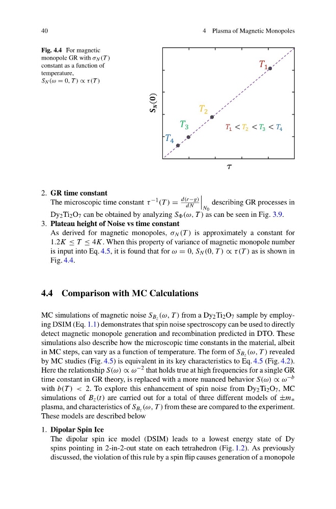
Fig. 4.4 For magnetic
monopole GR with σ N (T )
constant as a function of
temperature,
S N (ω = 0, T ) ∝ τ (T )
Ù
2. GR time constant
The microscopic time constant τ −1 (T ) =
d(r−g)
dN
N 0
describing GR processes in
Dy 2 Ti 2 O 7 can be obtained by analyzing S (ω, T ) as can be seen in Fig. 3.9.
3. Plateau height of Noise vs time constant
As derived for magnetic monopoles, σ N (T ) is approximately a constant for
1.2K ≤ T ≤ 4K. When this property of variance of magnetic monopole number
is input into Eq. 4.5, it is found that for ω = 0, S N (0, T ) ∝ τ (T ) as is shown in
Fig. 4.4.
4.4 Comparison with MC Calculations
MC simulations of magnetic noise S B z (ω, T ) from a Dy 2 Ti 2 O 7 sample by employing DSIM (Eq. 1.1) demonstrates that spin noise spectroscopy can be used to directly
detect magnetic monopole generation and recombination predicted in DTO. These
simulations also describe how the microscopic time constants in the material, albeit
in MC steps, can vary as a function of temperature. The form of S B z (ω, T ) revealed
by MC studies (Fig. 4.5) is equivalent in its key characteristics to Eq. 4.5 (Fig. 4.2).
Here the relationship S(ω) ∝ ω −2 that holds true at high frequencies for a single GR
time constant in GR theory, is replaced with a more nuanced behavior S(ω) ∝ ω −b
with b(T ) < 2. To explore this enhancement of spin noise from Dy 2 Ti 2 O 7 , MC
simulations of B z (t) are carried out for a total of three different models of ±m ∗
plasma, and characteristics of S B z (ω, T ) from these are compared to the experiment.
These models are described below
1. Dipolar Spin Ice
The dipolar spin ice model (DSIM) leads to a lowest energy state of Dy
spins pointing in 2-in-2-out state on each tetrahedron (Fig. 1.2). As previously
discussed, the violation of this rule by a spin flip causes generation of a monopole
4 Plasma of Magnetic Monopoles
Fig. 4.4 For magnetic
monopole GR with σ N (T )
constant as a function of
temperature,
S N (ω = 0, T ) ∝ τ (T )
Ù
2. GR time constant
The microscopic time constant τ −1 (T ) =
d(r−g)
dN
N 0
describing GR processes in
Dy 2 Ti 2 O 7 can be obtained by analyzing S (ω, T ) as can be seen in Fig. 3.9.
3. Plateau height of Noise vs time constant
As derived for magnetic monopoles, σ N (T ) is approximately a constant for
1.2K ≤ T ≤ 4K. When this property of variance of magnetic monopole number
is input into Eq. 4.5, it is found that for ω = 0, S N (0, T ) ∝ τ (T ) as is shown in
Fig. 4.4.
4.4 Comparison with MC Calculations
MC simulations of magnetic noise S B z (ω, T ) from a Dy 2 Ti 2 O 7 sample by employing DSIM (Eq. 1.1) demonstrates that spin noise spectroscopy can be used to directly
detect magnetic monopole generation and recombination predicted in DTO. These
simulations also describe how the microscopic time constants in the material, albeit
in MC steps, can vary as a function of temperature. The form of S B z (ω, T ) revealed
by MC studies (Fig. 4.5) is equivalent in its key characteristics to Eq. 4.5 (Fig. 4.2).
Here the relationship S(ω) ∝ ω −2 that holds true at high frequencies for a single GR
time constant in GR theory, is replaced with a more nuanced behavior S(ω) ∝ ω −b
with b(T ) < 2. To explore this enhancement of spin noise from Dy 2 Ti 2 O 7 , MC
simulations of B z (t) are carried out for a total of three different models of ±m ∗
plasma, and characteristics of S B z (ω, T ) from these are compared to the experiment.
These models are described below
1. Dipolar Spin Ice
The dipolar spin ice model (DSIM) leads to a lowest energy state of Dy
spins pointing in 2-in-2-out state on each tetrahedron (Fig. 1.2). As previously
discussed, the violation of this rule by a spin flip causes generation of a monopole