

38
4 Plasma of Magnetic Monopoles
4.2 Variance of Monopole Pair Number Fluctuations
We can deduce that generation recombination τ (T ) behaves in a manner that
matches our expectations from previous experiments. Decoding what σ N (T ) for
magnetic monopoles will shed further light on what Eq. 4.5 can reveal about
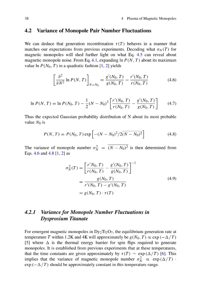
magnetic monopole noise. From Eq. 4.1, expanding ln P (N, T ) about its maximum
value ln P (N 0 , T ) in a quadratic fashion [1, 2] yields
∂ 2
∂N 2 ln P (N, T )
N =N 0
=
g (N 0 , T )
g(N 0 , T )
−
r (N 0 , T )
r(N 0 , T )
(4.6)
ln P (N, T ) = ln P (N 0 , T ) −
1
2
(N − N 0 )
2
r (N 0 , T )
r(N 0 , T )
−
g (N 0 , T )
g(N 0 , T )
(4.7)
Thus the expected Gaussian probability distribution of N about its most probable
value N 0 is
P (N, T ) = P (N 0 , T ) exp
−(N − N 0 )
2 /2(N − N 0 ) 2
(4.8)
The variance of monopole number σ 2
N = (N − N 0 ) 2 is then determined from
Eqs. 4.6 and 4.8 [1, 2] as
σ
2
N (T ) =
r N 0 , T )
r(N 0 , T )
−
g (N 0 , T )
g(N 0 , T )
−1
=
g(N 0 , T )
r (N 0 , T ) − g (N 0 , T )
= g(N 0 , T ) · τ (T )
(4.9)
4.2.1 Variance for Monopole Number Fluctuations in
Dysprosium Titanate
For emergent magnetic monopoles in Dy 2 Ti 2 O 7 , the equilibrium generation rate at
temperature T within 1.2K and 4K will approximately be g(N 0 , T ) ∝ exp (− )
[5] where is the thermal energy barrier for spin flips required to generate
monopoles. It is established from previous experiments that at these temperatures,
that the time constants are given approximately by τ (T ) ∼ exp ((/T ) [6]. This
implies that the variance of magnetic monopole number σ 2
N ∝ exp ((/T ) ·
exp (− ) should be approximately constant in this temperature range.
4 Plasma of Magnetic Monopoles
4.2 Variance of Monopole Pair Number Fluctuations
We can deduce that generation recombination τ (T ) behaves in a manner that
matches our expectations from previous experiments. Decoding what σ N (T ) for
magnetic monopoles will shed further light on what Eq. 4.5 can reveal about
magnetic monopole noise. From Eq. 4.1, expanding ln P (N, T ) about its maximum
value ln P (N 0 , T ) in a quadratic fashion [1, 2] yields
∂ 2
∂N 2 ln P (N, T )
N =N 0
=
g (N 0 , T )
g(N 0 , T )
−
r (N 0 , T )
r(N 0 , T )
(4.6)
ln P (N, T ) = ln P (N 0 , T ) −
1
2
(N − N 0 )
2
r (N 0 , T )
r(N 0 , T )
−
g (N 0 , T )
g(N 0 , T )
(4.7)
Thus the expected Gaussian probability distribution of N about its most probable
value N 0 is
P (N, T ) = P (N 0 , T ) exp
−(N − N 0 )
2 /2(N − N 0 ) 2
(4.8)
The variance of monopole number σ 2
N = (N − N 0 ) 2 is then determined from
Eqs. 4.6 and 4.8 [1, 2] as
σ
2
N (T ) =
r N 0 , T )
r(N 0 , T )
−
g (N 0 , T )
g(N 0 , T )
−1
=
g(N 0 , T )
r (N 0 , T ) − g (N 0 , T )
= g(N 0 , T ) · τ (T )
(4.9)
4.2.1 Variance for Monopole Number Fluctuations in
Dysprosium Titanate
For emergent magnetic monopoles in Dy 2 Ti 2 O 7 , the equilibrium generation rate at
temperature T within 1.2K and 4K will approximately be g(N 0 , T ) ∝ exp (− )
[5] where is the thermal energy barrier for spin flips required to generate
monopoles. It is established from previous experiments that at these temperatures,
that the time constants are given approximately by τ (T ) ∼ exp ((/T ) [6]. This
implies that the variance of magnetic monopole number σ 2
N ∝ exp ((/T ) ·
exp (− ) should be approximately constant in this temperature range.