

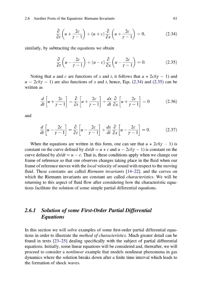
∂
∂t
u þ
2c
γ À 1
þ u þ c
ð
Þ
∂
∂x
u þ
2c
γ À 1
¼ 0,
ð2:34Þ
similarly, by subtracting the equations we obtain
∂
∂t
u À
2c
γ À 1
þ u À c
ð
Þ
∂
∂x
u À
2c
γ À 1
¼ 0:
ð2:35Þ
Noting that u and c are functions of x and t, it follows that u + 2c/(γ À 1) and
u À 2c/(γ À 1) are also functions of x and t, hence, Eqs. (2.34) and (2.35) can be
written as
d
dt
u þ
2c
γ À 1
!
¼
∂
∂t
u þ
2c
γ À 1
!
þ
dx
dt
∂
∂x
u þ
2c
γ À 1
!
¼ 0
ð2:36Þ
and
d
dt
u À
2c
γ À 1
!
¼
∂
∂t
u À
2c
γ À 1
!
þ
dx
dt
∂
∂x
u À
2c
γ À 1
!
¼ 0:
ð2:37Þ
When the equations are written in this form, one can see that u + 2c/(γ À 1) is
constant on the curve defined by dx/dt ¼ u + c and u À 2c/(γ À 1) is constant on the
curve defined by dx/dt ¼ u À c. That is, these conditions apply when we change our
frame of reference so that one observes changes taking place in the fluid when our
frame of reference moves with the local velocity of sound with respect to the moving
fluid. These constants are called Riemann invariants [14–22]. and the curves on
which the Riemann invariants are constant are called characteristics. We will be
returning to this aspect of fluid flow after considering how the characteristic equations facilitate the solution of some simple partial differential equations.
2.6.1 Solution of some First-Order Partial Differential
Equations
In this section we will solve examples of some first-order partial differential equations in order to illustrate the method of characteristics. Much greater detail can be
found in texts [23–25] dealing specifically with the subject of partial differential
equations. Initially, some linear equations will be considered and, thereafter, we will
proceed to consider a nonlinear example that models nonlinear phenomena in gas
dynamics where the solution breaks down after a finite time interval which leads to
the formation of shock waves.
2.6 Another Form of the Equations: Riemann Invariants
61
∂t
u þ
2c
γ À 1
þ u þ c
ð
Þ
∂
∂x
u þ
2c
γ À 1
¼ 0,
ð2:34Þ
similarly, by subtracting the equations we obtain
∂
∂t
u À
2c
γ À 1
þ u À c
ð
Þ
∂
∂x
u À
2c
γ À 1
¼ 0:
ð2:35Þ
Noting that u and c are functions of x and t, it follows that u + 2c/(γ À 1) and
u À 2c/(γ À 1) are also functions of x and t, hence, Eqs. (2.34) and (2.35) can be
written as
d
dt
u þ
2c
γ À 1
!
¼
∂
∂t
u þ
2c
γ À 1
!
þ
dx
dt
∂
∂x
u þ
2c
γ À 1
!
¼ 0
ð2:36Þ
and
d
dt
u À
2c
γ À 1
!
¼
∂
∂t
u À
2c
γ À 1
!
þ
dx
dt
∂
∂x
u À
2c
γ À 1
!
¼ 0:
ð2:37Þ
When the equations are written in this form, one can see that u + 2c/(γ À 1) is
constant on the curve defined by dx/dt ¼ u + c and u À 2c/(γ À 1) is constant on the
curve defined by dx/dt ¼ u À c. That is, these conditions apply when we change our
frame of reference so that one observes changes taking place in the fluid when our
frame of reference moves with the local velocity of sound with respect to the moving
fluid. These constants are called Riemann invariants [14–22]. and the curves on
which the Riemann invariants are constant are called characteristics. We will be
returning to this aspect of fluid flow after considering how the characteristic equations facilitate the solution of some simple partial differential equations.
2.6.1 Solution of some First-Order Partial Differential
Equations
In this section we will solve examples of some first-order partial differential equations in order to illustrate the method of characteristics. Much greater detail can be
found in texts [23–25] dealing specifically with the subject of partial differential
equations. Initially, some linear equations will be considered and, thereafter, we will
proceed to consider a nonlinear example that models nonlinear phenomena in gas
dynamics where the solution breaks down after a finite time interval which leads to
the formation of shock waves.
2.6 Another Form of the Equations: Riemann Invariants
61