

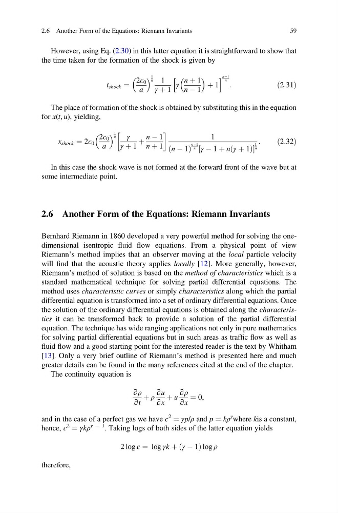
However, using Eq. (2.30) in this latter equation it is straightforward to show that
the time taken for the formation of the shock is given by
t shock ¼
2c 0
a
1
n
1
γ þ 1
γ
n þ 1
n À 1
þ 1
h
i nÀ1
n :
ð2:31Þ
The place of formation of the shock is obtained by substituting this in the equation
for x(t, u), yielding,
x shock ¼ 2c 0
2c 0
a
1
n
γ
γ þ 1
þ
n À 1
n þ 1
!
1
n À 1
ð
Þ
nÀ1
n γ À 1 þ n γ þ 1
ð
Þ
½
1
n
:
ð2:32Þ
In this case the shock wave is not formed at the forward front of the wave but at
some intermediate point.
2.6 Another Form of the Equations: Riemann Invariants
Bernhard Riemann in 1860 developed a very powerful method for solving the onedimensional isentropic fluid flow equations. From a physical point of view
Riemann’s method implies that an observer moving at the local particle velocity
will find that the acoustic theory applies locally [12]. More generally, however,
Riemann’s method of solution is based on the method of characteristics which is a
standard mathematical technique for solving partial differential equations. The
method uses characteristic curves or simply characteristics along which the partial
differential equation is transformed into a set of ordinary differential equations. Once
the solution of the ordinary differential equations is obtained along the characteristics it can be transformed back to provide a solution of the partial differential
equation. The technique has wide ranging applications not only in pure mathematics
for solving partial differential equations but in such areas as traffic flow as well as
fluid flow and a good starting point for the interested reader is the text by Whitham
[13]. Only a very brief outline of Riemann’s method is presented here and much
greater details can be found in the many references cited at the end of the chapter.
The continuity equation is
∂ρ
∂t
þ ρ
∂u
∂x
þ u
∂ρ
∂x
¼ 0,
and in the case of a perfect gas we have c
2
¼ γp/ρ and p ¼ kρ
γ where kis a constant,
hence, c
2
¼ γkρ
γ À 1 . Taking logs of both sides of the latter equation yields
2 log c ¼ log γk þ γ À 1
ð
Þlog ρ
therefore,
2.6 Another Form of the Equations: Riemann Invariants
59
the time taken for the formation of the shock is given by
t shock ¼
2c 0
a
1
n
1
γ þ 1
γ
n þ 1
n À 1
þ 1
h
i nÀ1
n :
ð2:31Þ
The place of formation of the shock is obtained by substituting this in the equation
for x(t, u), yielding,
x shock ¼ 2c 0
2c 0
a
1
n
γ
γ þ 1
þ
n À 1
n þ 1
!
1
n À 1
ð
Þ
nÀ1
n γ À 1 þ n γ þ 1
ð
Þ
½
1
n
:
ð2:32Þ
In this case the shock wave is not formed at the forward front of the wave but at
some intermediate point.
2.6 Another Form of the Equations: Riemann Invariants
Bernhard Riemann in 1860 developed a very powerful method for solving the onedimensional isentropic fluid flow equations. From a physical point of view
Riemann’s method implies that an observer moving at the local particle velocity
will find that the acoustic theory applies locally [12]. More generally, however,
Riemann’s method of solution is based on the method of characteristics which is a
standard mathematical technique for solving partial differential equations. The
method uses characteristic curves or simply characteristics along which the partial
differential equation is transformed into a set of ordinary differential equations. Once
the solution of the ordinary differential equations is obtained along the characteristics it can be transformed back to provide a solution of the partial differential
equation. The technique has wide ranging applications not only in pure mathematics
for solving partial differential equations but in such areas as traffic flow as well as
fluid flow and a good starting point for the interested reader is the text by Whitham
[13]. Only a very brief outline of Riemann’s method is presented here and much
greater details can be found in the many references cited at the end of the chapter.
The continuity equation is
∂ρ
∂t
þ ρ
∂u
∂x
þ u
∂ρ
∂x
¼ 0,
and in the case of a perfect gas we have c
2
¼ γp/ρ and p ¼ kρ
γ where kis a constant,
hence, c
2
¼ γkρ
γ À 1 . Taking logs of both sides of the latter equation yields
2 log c ¼ log γk þ γ À 1
ð
Þlog ρ
therefore,
2.6 Another Form of the Equations: Riemann Invariants
59