

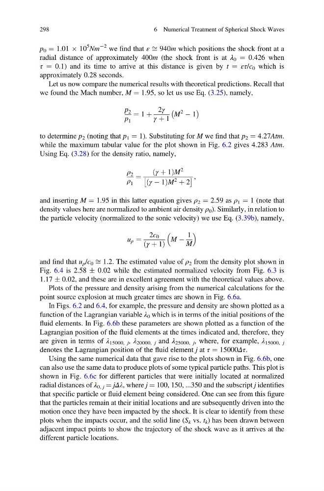
p 0 ¼ 1.01 Â 10
5 Nm
À2 we find that ε ffi 940m which positions the shock front at a
radial distance of approximately 400m (the shock front is at λ 0 ¼ 0.426 when
τ ¼ 0.1) and its time to arrive at this distance is given by t ¼ ετ/c 0 which is
approximately 0.28 seconds.
Let us now compare the numerical results with theoretical predictions. Recall that
we found the Mach number, M ¼ 1.95, so let us use Eq. (3.25), namely,
p 2
p 1
¼ 1 þ
2γ
γ þ 1
M
2
À 1
À
Á
to determine p 2 (noting that p 1 ¼ 1). Substituting for M we find that p 2 ¼ 4.27Atm.
while the maximum tabular value for the plot shown in Fig. 6.2 gives 4.283 Atm.
Using Eq. (3.28) for the density ratio, namely,
ρ 2
ρ 1
¼
γ þ 1
ð
ÞM
2
γ À 1
ð
ÞM
2
þ 2
Â
à ,
and inserting M ¼ 1.95 in this latter equation gives ρ 2 ¼ 2.59 as ρ 1 ¼ 1 (note that
density values here are normalized to ambient air density ρ 0 ). Similarly, in relation to
the particle velocity (normalized to the sonic velocity) we use Eq. (3.39b), namely,
u p ¼
2c 0
γ þ 1
ð
Þ
M À
1
M
and find that u p /c 0 ffi 1.2. The estimated value of ρ 2 from the density plot shown in
Fig. 6.4 is 2.58 Æ 0.02 while the estimated normalized velocity from Fig. 6.3 is
1.17 Æ 0.02, and these are in excellent agreement with the theoretical values above.
Plots of the pressure and density arising from the numerical calculations for the
point source explosion at much greater times are shown in Fig. 6.6a.
In Figs. 6.2 and 6.4, for example, the pressure and density are shown plotted as a
function of the Lagrangian variable λ 0 which is in terms of the initial positions of the
fluid elements. In Fig. 6.6b these parameters are shown plotted as a function of the
Lagrangian position of the fluid elements at the times indicated and, therefore, they
are given in terms of λ 15000, j , λ 20000, j and λ 25000, j , where, for example, λ 15000, j
denotes the Lagrangian position of the fluid element j at τ ¼ 15000Δτ.
Using the same numerical data that gave rise to the plots shown in Fig. 6.6b, one
can also use the same data to produce plots of some typical particle paths. This plot is
shown in Fig. 6.6c for different particles that were initially located at normalized
radial distances of λ 0, j ¼ jΔλ, where j ¼ 100, 150, ...350 and the subscript j identifies
that specific particle or fluid element being considered. One can see from this figure
that the particles remain at their initial locations and are subsequently driven into the
motion once they have been impacted by the shock. It is clear to identify from these
plots when the impacts occur, and the solid line (S k vs. t k ) has been drawn between
adjacent impact points to show the trajectory of the shock wave as it arrives at the
different particle locations.
298
6 Numerical Treatment of Spherical Shock Waves
5 Nm
À2 we find that ε ffi 940m which positions the shock front at a
radial distance of approximately 400m (the shock front is at λ 0 ¼ 0.426 when
τ ¼ 0.1) and its time to arrive at this distance is given by t ¼ ετ/c 0 which is
approximately 0.28 seconds.
Let us now compare the numerical results with theoretical predictions. Recall that
we found the Mach number, M ¼ 1.95, so let us use Eq. (3.25), namely,
p 2
p 1
¼ 1 þ
2γ
γ þ 1
M
2
À 1
À
Á
to determine p 2 (noting that p 1 ¼ 1). Substituting for M we find that p 2 ¼ 4.27Atm.
while the maximum tabular value for the plot shown in Fig. 6.2 gives 4.283 Atm.
Using Eq. (3.28) for the density ratio, namely,
ρ 2
ρ 1
¼
γ þ 1
ð
ÞM
2
γ À 1
ð
ÞM
2
þ 2
Â
à ,
and inserting M ¼ 1.95 in this latter equation gives ρ 2 ¼ 2.59 as ρ 1 ¼ 1 (note that
density values here are normalized to ambient air density ρ 0 ). Similarly, in relation to
the particle velocity (normalized to the sonic velocity) we use Eq. (3.39b), namely,
u p ¼
2c 0
γ þ 1
ð
Þ
M À
1
M
and find that u p /c 0 ffi 1.2. The estimated value of ρ 2 from the density plot shown in
Fig. 6.4 is 2.58 Æ 0.02 while the estimated normalized velocity from Fig. 6.3 is
1.17 Æ 0.02, and these are in excellent agreement with the theoretical values above.
Plots of the pressure and density arising from the numerical calculations for the
point source explosion at much greater times are shown in Fig. 6.6a.
In Figs. 6.2 and 6.4, for example, the pressure and density are shown plotted as a
function of the Lagrangian variable λ 0 which is in terms of the initial positions of the
fluid elements. In Fig. 6.6b these parameters are shown plotted as a function of the
Lagrangian position of the fluid elements at the times indicated and, therefore, they
are given in terms of λ 15000, j , λ 20000, j and λ 25000, j , where, for example, λ 15000, j
denotes the Lagrangian position of the fluid element j at τ ¼ 15000Δτ.
Using the same numerical data that gave rise to the plots shown in Fig. 6.6b, one
can also use the same data to produce plots of some typical particle paths. This plot is
shown in Fig. 6.6c for different particles that were initially located at normalized
radial distances of λ 0, j ¼ jΔλ, where j ¼ 100, 150, ...350 and the subscript j identifies
that specific particle or fluid element being considered. One can see from this figure
that the particles remain at their initial locations and are subsequently driven into the
motion once they have been impacted by the shock. It is clear to identify from these
plots when the impacts occur, and the solid line (S k vs. t k ) has been drawn between
adjacent impact points to show the trajectory of the shock wave as it arrives at the
different particle locations.
298
6 Numerical Treatment of Spherical Shock Waves