

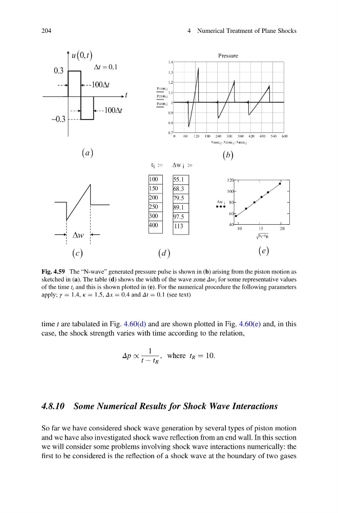
time t are tabulated in Fig. 4.60(d) and are shown plotted in Fig. 4.60(e) and, in this
case, the shock strength varies with time according to the relation,
Δp /
1
t À t R
, where t R ¼ 10:
4.8.10 Some Numerical Results for Shock Wave Interactions
So far we have considered shock wave generation by several types of piston motion
and we have also investigated shock wave reflection from an end wall. In this section
we will consider some problems involving shock wave interactions numerically: the
first to be considered is the reflection of a shock wave at the boundary of two gases
Fig. 4.59 The “N-wave” generated pressure pulse is shown in (b) arising from the piston motion as
sketched in (a). The table (d) shows the width of the wave zone Δw i for some representative values
of the time t i and this is shown plotted in (e). For the numerical procedure the following parameters
apply; γ ¼ 1.4, κ ¼ 1.5, Δx ¼ 0.4 and Δt ¼ 0.1 (see text)
204
4 Numerical Treatment of Plane Shocks
case, the shock strength varies with time according to the relation,
Δp /
1
t À t R
, where t R ¼ 10:
4.8.10 Some Numerical Results for Shock Wave Interactions
So far we have considered shock wave generation by several types of piston motion
and we have also investigated shock wave reflection from an end wall. In this section
we will consider some problems involving shock wave interactions numerically: the
first to be considered is the reflection of a shock wave at the boundary of two gases
Fig. 4.59 The “N-wave” generated pressure pulse is shown in (b) arising from the piston motion as
sketched in (a). The table (d) shows the width of the wave zone Δw i for some representative values
of the time t i and this is shown plotted in (e). For the numerical procedure the following parameters
apply; γ ¼ 1.4, κ ¼ 1.5, Δx ¼ 0.4 and Δt ¼ 0.1 (see text)
204
4 Numerical Treatment of Plane Shocks