

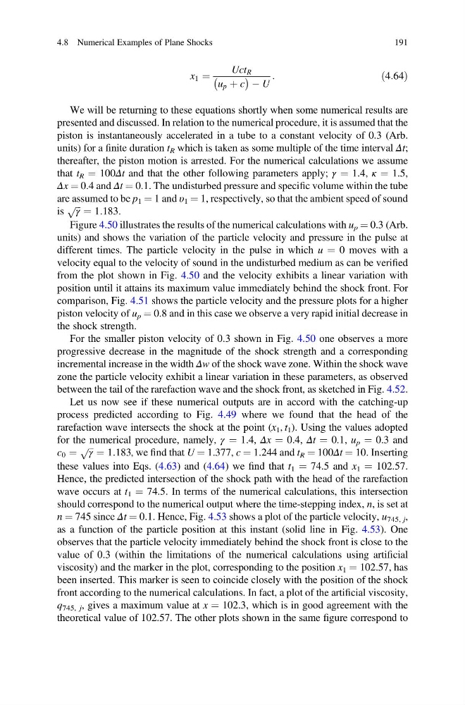
x 1 ¼
Uct R
u p þ c
À
Á À U
:
ð4:64Þ
We will be returning to these equations shortly when some numerical results are
presented and discussed. In relation to the numerical procedure, it is assumed that the
piston is instantaneously accelerated in a tube to a constant velocity of 0.3 (Arb.
units) for a finite duration t R which is taken as some multiple of the time interval Δt;
thereafter, the piston motion is arrested. For the numerical calculations we assume
that t R ¼ 100Δt and that the other following parameters apply; γ ¼ 1.4, κ ¼ 1.5,
Δx ¼ 0.4 and Δt ¼ 0.1. The undisturbed pressure and specific volume within the tube
are assumed to be p 1 ¼ 1 and υ 1 ¼ 1, respectively, so that the ambient speed of sound
is
ffiffi ffi
γ
p ¼ 1:183.
Figure 4.50 illustrates the results of the numerical calculations with u p ¼ 0.3 (Arb.
units) and shows the variation of the particle velocity and pressure in the pulse at
different times. The particle velocity in the pulse in which u ¼ 0 moves with a
velocity equal to the velocity of sound in the undisturbed medium as can be verified
from the plot shown in Fig. 4.50 and the velocity exhibits a linear variation with
position until it attains its maximum value immediately behind the shock front. For
comparison, Fig. 4.51 shows the particle velocity and the pressure plots for a higher
piston velocity of u p ¼ 0.8 and in this case we observe a very rapid initial decrease in
the shock strength.
For the smaller piston velocity of 0.3 shown in Fig. 4.50 one observes a more
progressive decrease in the magnitude of the shock strength and a corresponding
incremental increase in the width Δw of the shock wave zone. Within the shock wave
zone the particle velocity exhibit a linear variation in these parameters, as observed
between the tail of the rarefaction wave and the shock front, as sketched in Fig. 4.52.
Let us now see if these numerical outputs are in accord with the catching-up
process predicted according to Fig. 4.49 where we found that the head of the
rarefaction wave intersects the shock at the point (x 1 , t 1 ). Using the values adopted
for the numerical procedure, namely, γ ¼ 1.4, Δx ¼ 0.4, Δt ¼ 0.1, u p ¼ 0.3 and
c 0 ¼
ffiffi ffi
γ
p ¼ 1:183, we find that U ¼ 1.377, c ¼ 1.244 and t R ¼ 100Δt ¼ 10. Inserting
these values into Eqs. (4.63) and (4.64) we find that t 1 ¼ 74.5 and x 1 ¼ 102.57.
Hence, the predicted intersection of the shock path with the head of the rarefaction
wave occurs at t 1 ¼ 74.5. In terms of the numerical calculations, this intersection
should correspond to the numerical output where the time-stepping index, n, is set at
n ¼ 745 since Δt ¼ 0.1. Hence, Fig. 4.53 shows a plot of the particle velocity, u 745, j ,
as a function of the particle position at this instant (solid line in Fig. 4.53). One
observes that the particle velocity immediately behind the shock front is close to the
value of 0.3 (within the limitations of the numerical calculations using artificial
viscosity) and the marker in the plot, corresponding to the position x 1 ¼ 102.57, has
been inserted. This marker is seen to coincide closely with the position of the shock
front according to the numerical calculations. In fact, a plot of the artificial viscosity,
q 745, j , gives a maximum value at x ¼ 102.3, which is in good agreement with the
theoretical value of 102.57. The other plots shown in the same figure correspond to
4.8 Numerical Examples of Plane Shocks
191
Uct R
u p þ c
À
Á À U
:
ð4:64Þ
We will be returning to these equations shortly when some numerical results are
presented and discussed. In relation to the numerical procedure, it is assumed that the
piston is instantaneously accelerated in a tube to a constant velocity of 0.3 (Arb.
units) for a finite duration t R which is taken as some multiple of the time interval Δt;
thereafter, the piston motion is arrested. For the numerical calculations we assume
that t R ¼ 100Δt and that the other following parameters apply; γ ¼ 1.4, κ ¼ 1.5,
Δx ¼ 0.4 and Δt ¼ 0.1. The undisturbed pressure and specific volume within the tube
are assumed to be p 1 ¼ 1 and υ 1 ¼ 1, respectively, so that the ambient speed of sound
is
ffiffi ffi
γ
p ¼ 1:183.
Figure 4.50 illustrates the results of the numerical calculations with u p ¼ 0.3 (Arb.
units) and shows the variation of the particle velocity and pressure in the pulse at
different times. The particle velocity in the pulse in which u ¼ 0 moves with a
velocity equal to the velocity of sound in the undisturbed medium as can be verified
from the plot shown in Fig. 4.50 and the velocity exhibits a linear variation with
position until it attains its maximum value immediately behind the shock front. For
comparison, Fig. 4.51 shows the particle velocity and the pressure plots for a higher
piston velocity of u p ¼ 0.8 and in this case we observe a very rapid initial decrease in
the shock strength.
For the smaller piston velocity of 0.3 shown in Fig. 4.50 one observes a more
progressive decrease in the magnitude of the shock strength and a corresponding
incremental increase in the width Δw of the shock wave zone. Within the shock wave
zone the particle velocity exhibit a linear variation in these parameters, as observed
between the tail of the rarefaction wave and the shock front, as sketched in Fig. 4.52.
Let us now see if these numerical outputs are in accord with the catching-up
process predicted according to Fig. 4.49 where we found that the head of the
rarefaction wave intersects the shock at the point (x 1 , t 1 ). Using the values adopted
for the numerical procedure, namely, γ ¼ 1.4, Δx ¼ 0.4, Δt ¼ 0.1, u p ¼ 0.3 and
c 0 ¼
ffiffi ffi
γ
p ¼ 1:183, we find that U ¼ 1.377, c ¼ 1.244 and t R ¼ 100Δt ¼ 10. Inserting
these values into Eqs. (4.63) and (4.64) we find that t 1 ¼ 74.5 and x 1 ¼ 102.57.
Hence, the predicted intersection of the shock path with the head of the rarefaction
wave occurs at t 1 ¼ 74.5. In terms of the numerical calculations, this intersection
should correspond to the numerical output where the time-stepping index, n, is set at
n ¼ 745 since Δt ¼ 0.1. Hence, Fig. 4.53 shows a plot of the particle velocity, u 745, j ,
as a function of the particle position at this instant (solid line in Fig. 4.53). One
observes that the particle velocity immediately behind the shock front is close to the
value of 0.3 (within the limitations of the numerical calculations using artificial
viscosity) and the marker in the plot, corresponding to the position x 1 ¼ 102.57, has
been inserted. This marker is seen to coincide closely with the position of the shock
front according to the numerical calculations. In fact, a plot of the artificial viscosity,
q 745, j , gives a maximum value at x ¼ 102.3, which is in good agreement with the
theoretical value of 102.57. The other plots shown in the same figure correspond to
4.8 Numerical Examples of Plane Shocks
191