

speed was given by u(t, 0) ¼ 0.3 which is approximately 30% of the speed of sound
(equal to
ffiffi ffi
γ
p ¼ 1:18 as the ambient pressure and density have unity values) and we
found that a shock wave formed immediately and raced ahead of the piston with a
velocity of 1.38 (Arb. units). Let us now reduce the piston velocity to about 0.03% of
the sound speed so that u(t, 0) ¼ 0.0003. By carrying out the numerical calculations
with this reduced value of u(t, 0), one can obtain plots of the particle velocity as a
function of position for the three different times as shown in Fig. 4.43. These plots
should be compared with the velocity plots shown in Fig. 4.17 where the velocity
was taken as u(t, 0) ¼ 0.3. The magnitude of the piston’s velocity is the only
difference in the programs generating the numerical outputs shown in Figs. 4.21
and 4.43. The important point to note from Fig. 4.43 is that the piston-generated
disturbance (represented by, for example, the plot for u 1000, j ) propagates at the speed
of sound which can be verified from the numerical values shown in Fig. 4.43.
We have already noted that the magnitude of the velocity of the shock wave in the
plot shown in Fig. 4.17 was found to be approximately 1.38 (Arb. units). This value
was confirmed by using Eq. (3.40) in Chap. 3 which explicitly includes the velocity
of the piston motion in addition to the velocity of sound. We could of course use the
same equation to confirm the velocity of the disturbance in the case of the plot shown
in Fig. 4.43 in which the piston’s velocity is considerably reduced. On the other
hand, let us for the moment disregard any knowledge of the material presented in
Chap. 3 or, for that matter, any knowledge in relation to the speed of propagation of
small-amplitude disturbances that was discussed in Section 1.8 where the speed of
sound c 0 appears explicitly. Hence, by disregarding this knowledge, it is interesting
to note that the equations summarized in Sect. 4.5.1, or their equivalent difference
equations which are used in the numerical calculations, makes no explicit reference
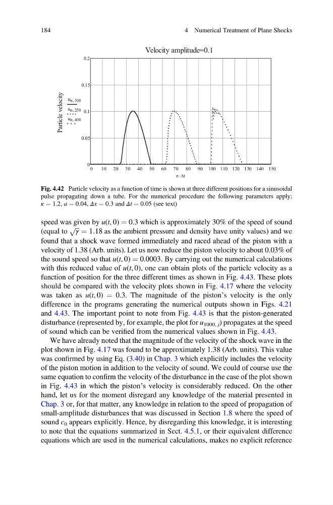
Fig. 4.42 Particle velocity as a function of time is shown at three different positions for a sinusoidal
pulse propagating down a tube. For the numerical procedure the following parameters apply;
κ ¼ 1.2, a ¼ 0.04, Δx ¼ 0.3 and Δt ¼ 0.05 (see text)
184
4 Numerical Treatment of Plane Shocks
(equal to
ffiffi ffi
γ
p ¼ 1:18 as the ambient pressure and density have unity values) and we
found that a shock wave formed immediately and raced ahead of the piston with a
velocity of 1.38 (Arb. units). Let us now reduce the piston velocity to about 0.03% of
the sound speed so that u(t, 0) ¼ 0.0003. By carrying out the numerical calculations
with this reduced value of u(t, 0), one can obtain plots of the particle velocity as a
function of position for the three different times as shown in Fig. 4.43. These plots
should be compared with the velocity plots shown in Fig. 4.17 where the velocity
was taken as u(t, 0) ¼ 0.3. The magnitude of the piston’s velocity is the only
difference in the programs generating the numerical outputs shown in Figs. 4.21
and 4.43. The important point to note from Fig. 4.43 is that the piston-generated
disturbance (represented by, for example, the plot for u 1000, j ) propagates at the speed
of sound which can be verified from the numerical values shown in Fig. 4.43.
We have already noted that the magnitude of the velocity of the shock wave in the
plot shown in Fig. 4.17 was found to be approximately 1.38 (Arb. units). This value
was confirmed by using Eq. (3.40) in Chap. 3 which explicitly includes the velocity
of the piston motion in addition to the velocity of sound. We could of course use the
same equation to confirm the velocity of the disturbance in the case of the plot shown
in Fig. 4.43 in which the piston’s velocity is considerably reduced. On the other
hand, let us for the moment disregard any knowledge of the material presented in
Chap. 3 or, for that matter, any knowledge in relation to the speed of propagation of
small-amplitude disturbances that was discussed in Section 1.8 where the speed of
sound c 0 appears explicitly. Hence, by disregarding this knowledge, it is interesting
to note that the equations summarized in Sect. 4.5.1, or their equivalent difference
equations which are used in the numerical calculations, makes no explicit reference
Fig. 4.42 Particle velocity as a function of time is shown at three different positions for a sinusoidal
pulse propagating down a tube. For the numerical procedure the following parameters apply;
κ ¼ 1.2, a ¼ 0.04, Δx ¼ 0.3 and Δt ¼ 0.05 (see text)
184
4 Numerical Treatment of Plane Shocks