

(a) Initial conditions
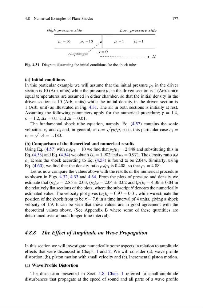
In this particular example we will assume that the initial pressure p 4 in the driver
section is 10 (Arb. units) while the pressure p 1 in the driven section is 1 (Arb. unit):
equal temperatures are assumed in either chamber, so that the initial density in the
driver section is 10 (Arb. units) while the initial density in the driven section is
1 (Arb. unit) as illustrated in Fig. 4.31. The air in both sections is initially at rest.
Assuming the following parameters apply for the numerical procedure; γ ¼ 1.4,
κ ¼ 1.2, Δx ¼ 0.1 and Δt ¼ 0.01.
The fundamental shock tube equation, namely, Eq. (4.57) contains the sonic
velocities c 1 and c 4 and, in general, as c ¼
ffiffiffiffiffiffiffiffiffi ffi
γp=ρ
p
, so in this particular case c 1 ¼
c 4 ¼
ffiffiffiffiffiffi ffi
1:4
p
¼ 1:183.
(b) Comparison of the theoretical and numerical results
Using Eq. (4.57) with p 4 /p 1 ¼ 10 we find that p 2 /p 1 ¼ 2.848 and substituting this in
Eq. (4.53) and Eq. (4.54) we obtain U s ¼ 1.902 and u 2 ¼ 0.971. The density ratio ρ 2 /
ρ 1 across the shock according to Eq. (4.58) is found to be 2.044. Similarly, using
Eq. (4.60), we find that the density ratio ρ 3 /ρ 4 is 0.408, so that ρ 3 ¼ 4.08.
Let us now compare the values above with the results of the numerical procedure
as shown in Figs. 4.32, 4.33 and 4.34. From the plots of pressure and density we
estimate that (p 2 ) N ¼ 2.85 Æ 0.03, (ρ 2 ) N ¼ 2.04 Æ 0.02 and (ρ 3 ) N ¼ 4.06 Æ 0.04 in
the relatively flat sections of the plots, where the subscript N denotes the numerically
estimated value. The velocity plot gives (u 2 ) N ¼ 0.97 Æ 0.01, while we estimate the
position of the shock front to be x ¼ 7.6 in a time interval of 4 units, giving a shock
velocity of 1.9. It can be seen that these values are in good agreement with the
theoretical values above. (See Appendix B where some of these quantities are
determined over a much longer time interval).
4.8.8 The Effect of Amplitude on Wave Propagation
In this section we will investigate numerically some aspects in relation to amplitude
effects that were discussed in Chaps. 1 and 2. We will consider (a), wave profile
distortion, (b), piston motion with small velocity and (c), incremental piston motion.
(a) Wave Profile Distortion
The discussion presented in Sect. 1.8, Chap. 1 referred to small-amplitude
disturbances that propagate at the speed of sound and all parts of a wave profile
Fig. 4.31 Diagram illustrating the initial conditions for the shock tube
4.8 Numerical Examples of Plane Shocks
177
In this particular example we will assume that the initial pressure p 4 in the driver
section is 10 (Arb. units) while the pressure p 1 in the driven section is 1 (Arb. unit):
equal temperatures are assumed in either chamber, so that the initial density in the
driver section is 10 (Arb. units) while the initial density in the driven section is
1 (Arb. unit) as illustrated in Fig. 4.31. The air in both sections is initially at rest.
Assuming the following parameters apply for the numerical procedure; γ ¼ 1.4,
κ ¼ 1.2, Δx ¼ 0.1 and Δt ¼ 0.01.
The fundamental shock tube equation, namely, Eq. (4.57) contains the sonic
velocities c 1 and c 4 and, in general, as c ¼
ffiffiffiffiffiffiffiffiffi ffi
γp=ρ
p
, so in this particular case c 1 ¼
c 4 ¼
ffiffiffiffiffiffi ffi
1:4
p
¼ 1:183.
(b) Comparison of the theoretical and numerical results
Using Eq. (4.57) with p 4 /p 1 ¼ 10 we find that p 2 /p 1 ¼ 2.848 and substituting this in
Eq. (4.53) and Eq. (4.54) we obtain U s ¼ 1.902 and u 2 ¼ 0.971. The density ratio ρ 2 /
ρ 1 across the shock according to Eq. (4.58) is found to be 2.044. Similarly, using
Eq. (4.60), we find that the density ratio ρ 3 /ρ 4 is 0.408, so that ρ 3 ¼ 4.08.
Let us now compare the values above with the results of the numerical procedure
as shown in Figs. 4.32, 4.33 and 4.34. From the plots of pressure and density we
estimate that (p 2 ) N ¼ 2.85 Æ 0.03, (ρ 2 ) N ¼ 2.04 Æ 0.02 and (ρ 3 ) N ¼ 4.06 Æ 0.04 in
the relatively flat sections of the plots, where the subscript N denotes the numerically
estimated value. The velocity plot gives (u 2 ) N ¼ 0.97 Æ 0.01, while we estimate the
position of the shock front to be x ¼ 7.6 in a time interval of 4 units, giving a shock
velocity of 1.9. It can be seen that these values are in good agreement with the
theoretical values above. (See Appendix B where some of these quantities are
determined over a much longer time interval).
4.8.8 The Effect of Amplitude on Wave Propagation
In this section we will investigate numerically some aspects in relation to amplitude
effects that were discussed in Chaps. 1 and 2. We will consider (a), wave profile
distortion, (b), piston motion with small velocity and (c), incremental piston motion.
(a) Wave Profile Distortion
The discussion presented in Sect. 1.8, Chap. 1 referred to small-amplitude
disturbances that propagate at the speed of sound and all parts of a wave profile
Fig. 4.31 Diagram illustrating the initial conditions for the shock tube
4.8 Numerical Examples of Plane Shocks
177