

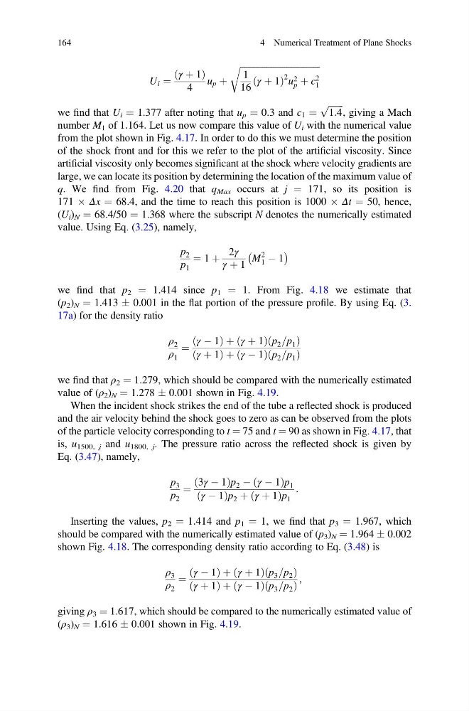
U i ¼
γ þ 1
ð
Þ
4
u p þ
ffiffiffiffiffiffiffiffiffiffiffiffiffiffiffiffiffiffiffiffiffiffiffiffiffiffiffiffiffiffiffiffiffiffiffiffi
1
16
γ þ 1
ð
Þ
2 u 2
p þ c 2
1
r
we find that U i ¼ 1.377 after noting that u p ¼ 0.3 and c 1 ¼
ffiffiffiffiffiffi ffi
1:4
p
, giving a Mach
number M 1 of 1.164. Let us now compare this value of U i with the numerical value
from the plot shown in Fig. 4.17. In order to do this we must determine the position
of the shock front and for this we refer to the plot of the artificial viscosity. Since
artificial viscosity only becomes significant at the shock where velocity gradients are
large, we can locate its position by determining the location of the maximum value of
q. We find from Fig. 4.20 that q Max occurs at j ¼ 171, so its position is
171 Â Δx ¼ 68.4, and the time to reach this position is 1000 Â Δt ¼ 50, hence,
(U i ) N ¼ 68.4/50 ¼ 1.368 where the subscript N denotes the numerically estimated
value. Using Eq. (3.25), namely,
p 2
p 1
¼ 1 þ
2γ
γ þ 1
M
2
1 À 1
À
Á
we find that p 2 ¼ 1.414 since p 1 ¼ 1. From Fig. 4.18 we estimate that
(p 2 ) N ¼ 1.413 Æ 0.001 in the flat portion of the pressure profile. By using Eq. (3.
17a) for the density ratio
ρ 2
ρ 1
¼
γ À 1
ð
Þþ γ þ 1
ð
Þ p 2 =p 1
ð
Þ
γ þ 1
ð
Þþ γ À 1
ð
Þ p 2 =p 1
ð
Þ
we find that ρ 2 ¼ 1.279, which should be compared with the numerically estimated
value of (ρ 2 ) N ¼ 1.278 Æ 0.001 shown in Fig. 4.19.
When the incident shock strikes the end of the tube a reflected shock is produced
and the air velocity behind the shock goes to zero as can be observed from the plots
of the particle velocity corresponding to t ¼ 75 and t ¼ 90 as shown in Fig. 4.17, that
is, u 1500, j and u 1800, j . The pressure ratio across the reflected shock is given by
Eq. (3.47), namely,
p 3
p 2
¼
3γ À 1
ð
Þp 2 À γ À 1
ð
Þp 1
γ À 1
ð
Þp 2 þ γ þ 1
ð
Þp 1
:
Inserting the values, p 2 ¼ 1.414 and p 1 ¼ 1, we find that p 3 ¼ 1.967, which
should be compared with the numerically estimated value of (p 3 ) N ¼ 1.964 Æ 0.002
shown Fig. 4.18. The corresponding density ratio according to Eq. (3.48) is
ρ 3
ρ 2
¼
γ À 1
ð
Þþ γ þ 1
ð
Þ p 3 =p 2
ð
Þ
γ þ 1
ð
Þþ γ À 1
ð
Þ p 3 =p 2
ð
Þ
,
giving ρ 3 ¼ 1.617, which should be compared to the numerically estimated value of
(ρ 3 ) N ¼ 1.616 Æ 0.001 shown in Fig. 4.19.
164
4 Numerical Treatment of Plane Shocks
γ þ 1
ð
Þ
4
u p þ
ffiffiffiffiffiffiffiffiffiffiffiffiffiffiffiffiffiffiffiffiffiffiffiffiffiffiffiffiffiffiffiffiffiffiffiffi
1
16
γ þ 1
ð
Þ
2 u 2
p þ c 2
1
r
we find that U i ¼ 1.377 after noting that u p ¼ 0.3 and c 1 ¼
ffiffiffiffiffiffi ffi
1:4
p
, giving a Mach
number M 1 of 1.164. Let us now compare this value of U i with the numerical value
from the plot shown in Fig. 4.17. In order to do this we must determine the position
of the shock front and for this we refer to the plot of the artificial viscosity. Since
artificial viscosity only becomes significant at the shock where velocity gradients are
large, we can locate its position by determining the location of the maximum value of
q. We find from Fig. 4.20 that q Max occurs at j ¼ 171, so its position is
171 Â Δx ¼ 68.4, and the time to reach this position is 1000 Â Δt ¼ 50, hence,
(U i ) N ¼ 68.4/50 ¼ 1.368 where the subscript N denotes the numerically estimated
value. Using Eq. (3.25), namely,
p 2
p 1
¼ 1 þ
2γ
γ þ 1
M
2
1 À 1
À
Á
we find that p 2 ¼ 1.414 since p 1 ¼ 1. From Fig. 4.18 we estimate that
(p 2 ) N ¼ 1.413 Æ 0.001 in the flat portion of the pressure profile. By using Eq. (3.
17a) for the density ratio
ρ 2
ρ 1
¼
γ À 1
ð
Þþ γ þ 1
ð
Þ p 2 =p 1
ð
Þ
γ þ 1
ð
Þþ γ À 1
ð
Þ p 2 =p 1
ð
Þ
we find that ρ 2 ¼ 1.279, which should be compared with the numerically estimated
value of (ρ 2 ) N ¼ 1.278 Æ 0.001 shown in Fig. 4.19.
When the incident shock strikes the end of the tube a reflected shock is produced
and the air velocity behind the shock goes to zero as can be observed from the plots
of the particle velocity corresponding to t ¼ 75 and t ¼ 90 as shown in Fig. 4.17, that
is, u 1500, j and u 1800, j . The pressure ratio across the reflected shock is given by
Eq. (3.47), namely,
p 3
p 2
¼
3γ À 1
ð
Þp 2 À γ À 1
ð
Þp 1
γ À 1
ð
Þp 2 þ γ þ 1
ð
Þp 1
:
Inserting the values, p 2 ¼ 1.414 and p 1 ¼ 1, we find that p 3 ¼ 1.967, which
should be compared with the numerically estimated value of (p 3 ) N ¼ 1.964 Æ 0.002
shown Fig. 4.18. The corresponding density ratio according to Eq. (3.48) is
ρ 3
ρ 2
¼
γ À 1
ð
Þþ γ þ 1
ð
Þ p 3 =p 2
ð
Þ
γ þ 1
ð
Þþ γ À 1
ð
Þ p 3 =p 2
ð
Þ
,
giving ρ 3 ¼ 1.617, which should be compared to the numerically estimated value of
(ρ 3 ) N ¼ 1.616 Æ 0.001 shown in Fig. 4.19.
164
4 Numerical Treatment of Plane Shocks