

4.8.2 Linear Ramp
Let us consider again the piston motion in a tube but, in this instance, we will assume
that the piston is uniformly accelerated to a constant speed according to the
equations;
u 0, t
ð Þ ¼ at ; 1 ! t ! 0
u 0, t
ð Þ ¼ 1; t > 1
as illustrated in Fig. 4.12. In addition to the piston motion, the following values were
chosen for the numerical procedure: Δx ¼ 0.3, Δt ¼ 0.05, γ ¼ 1.4 and κ ¼ 1.2. Let us
assume that the initial pressure and specific volume in the tube have the following
arbitrary values; p(x, 0) ¼ 1 and υ(x, 0) ¼ 1.
The particle velocity as a function of position is shown in Figs. 4.13 and 4.14 at
different times. The broken line in these plots indicates the time taken for the shock
wave to form according to Eq. (2.26) where we observe that the forward front begins
to takes on a vertical profile. In fact, Fig. 4.13 should be taken in conjunction with
Fig. 2.8 to compare the similarity between the numerical and analytical results.
Using Eq. (2.26), namely,
t shock ¼
2c 0
γ þ 1
ð
Þa
and noting that c 0 ¼
ffiffi ffi
γ
p as both the initial pressure and specific volume are unity, we
find that the time taken for the shock to form is t shock ¼ 98.6 (Arb. units). For times
less that this value one can easily verify from the plots that the forward front of the
6.8
6.85
6.9
6.95
7
0
0.1
0.2
0.3
0.4
t = 5
x
0.7
0.72
0.74
0.76
0.78
0.8
0
0.1
0.2
0.3
0.4
Time
Fluid Velocity
Fluid Velocity
x = 1
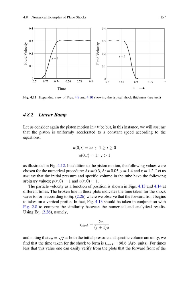
Fig. 4.11 Expanded view of Figs. 4.9 and 4.10 showing the typical shock thickness (see text)
4.8 Numerical Examples of Plane Shocks
157
Let us consider again the piston motion in a tube but, in this instance, we will assume
that the piston is uniformly accelerated to a constant speed according to the
equations;
u 0, t
ð Þ ¼ at ; 1 ! t ! 0
u 0, t
ð Þ ¼ 1; t > 1
as illustrated in Fig. 4.12. In addition to the piston motion, the following values were
chosen for the numerical procedure: Δx ¼ 0.3, Δt ¼ 0.05, γ ¼ 1.4 and κ ¼ 1.2. Let us
assume that the initial pressure and specific volume in the tube have the following
arbitrary values; p(x, 0) ¼ 1 and υ(x, 0) ¼ 1.
The particle velocity as a function of position is shown in Figs. 4.13 and 4.14 at
different times. The broken line in these plots indicates the time taken for the shock
wave to form according to Eq. (2.26) where we observe that the forward front begins
to takes on a vertical profile. In fact, Fig. 4.13 should be taken in conjunction with
Fig. 2.8 to compare the similarity between the numerical and analytical results.
Using Eq. (2.26), namely,
t shock ¼
2c 0
γ þ 1
ð
Þa
and noting that c 0 ¼
ffiffi ffi
γ
p as both the initial pressure and specific volume are unity, we
find that the time taken for the shock to form is t shock ¼ 98.6 (Arb. units). For times
less that this value one can easily verify from the plots that the forward front of the
6.8
6.85
6.9
6.95
7
0
0.1
0.2
0.3
0.4
t = 5
x
0.7
0.72
0.74
0.76
0.78
0.8
0
0.1
0.2
0.3
0.4
Time
Fluid Velocity
Fluid Velocity
x = 1
Fig. 4.11 Expanded view of Figs. 4.9 and 4.10 showing the typical shock thickness (see text)
4.8 Numerical Examples of Plane Shocks
157