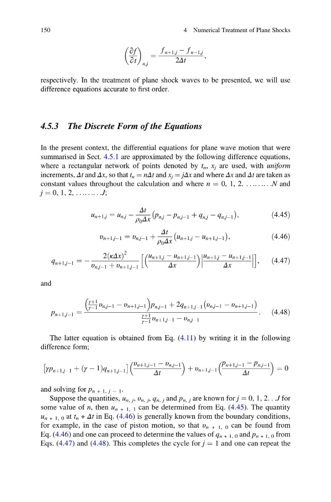
∂f
∂t
n,j
¼
f nþ1,j À f nÀ1,j
2Δt
,
respectively. In the treatment of plane shock waves to be presented, we will use
difference equations accurate to first order.
4.5.3 The Discrete Form of the Equations
In the present context, the differential equations for plane wave motion that were
summarised in Sect. 4.5.1 are approximated by the following difference equations,
where a rectangular network of points denoted by t n , x j are used, with uniform
increments, Δt and Δx, so that t n ¼ nΔt and x j ¼ jΔx and where Δx and Δt are taken as
constant values throughout the calculation and where n ¼ 0, 1, 2. . . .. . .. . .N and
j ¼ 0, 1, 2, . . .. . .. . .J;
u nþ1,j ¼ u n,j À
Δt
ρ 0 Δx
p n,j À p n,jÀ1 þ q n,j À q n,jÀ1
À
Á
,
ð4:45Þ
υ nþ1,jÀ1 ¼ υ n,jÀ1 þ
Δt
ρ 0 Δx
u nþ1,j À u nþ1,jÀ1
À
Á
,
ð4:46Þ
q nþ1,jÀ1 ¼ À
2 κΔx
ð
Þ
2
υ n,jÀ1 þ υ nþ1,jÀ1
u nþ1,j À u nþ1,jÀ1
Δx
u nþ1,j À u nþ1,jÀ1
Δx
h
i
,
ð4:47Þ
and
p nþ1,jÀ1 ¼
γþ1
γÀ1 υ n,jÀ1 À υ nþ1,jÀ1
p n,jÀ1 þ 2q nþ1,jÀ1 υ n,jÀ1 À υ nþ1,jÀ1
À
Á
γþ1
γÀ1 υ nþ1,jÀ1 À υ n,jÀ1
: ð4:48Þ
The latter equation is obtained from Eq. (4.11) by writing it in the following
difference form;
γp nþ1,jÀ1 þ γ À 1
ð
Þq nþ1,jÀ1
Â
à υ nþ1,jÀ1 À υ n,jÀ1
Δt
þ υ nþ1,jÀ1
p nþ1,jÀ1 À p n,jÀ1
Δt
¼ 0
and solving for p n + 1, j À 1 .
Suppose the quantities, u n, j , υ n, j , q n, j and p n, j are known for j ¼ 0, 1, 2. . .J for
some value of n, then u n + 1, 1 can be determined from Eq. (4.45). The quantity
u n + 1, 0 at t n + Δt in Eq. (4.46) is generally known from the boundary conditions,
for example, in the case of piston motion, so that υ n + 1, 0 can be found from
Eq. (4.46) and one can proceed to determine the values of q n + 1, 0 and p n + 1, 0 from
Eqs. (4.47) and (4.48). This completes the cycle for j ¼ 1 and one can repeat the
150
4 Numerical Treatment of Plane Shocks