

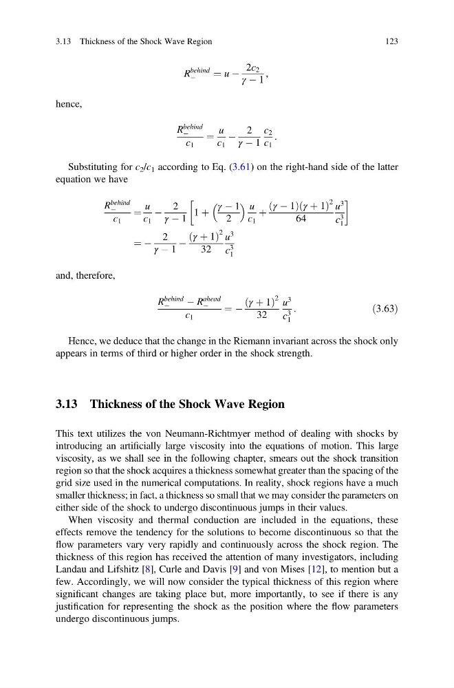
R
behind
À
¼ u À
2c 2
γ À 1
,
hence,
R
behind
À
c 1
¼
u
c 1
À
2
γ À 1
c 2
c 1
:
Substituting for c 2 /c 1 according to Eq. (3.61) on the right-hand side of the latter
equation we have
R
behind
À
c 1
¼
u
c 1
À
2
γ À 1
1 þ
γ À 1
2
u
c 1
þ
γ À 1
ð
Þ γ þ 1
ð
Þ
2
64
u
3
c
3
1
!
¼ À
2
γ À 1
À
γ þ 1
ð
Þ
2
32
u
3
c
3
1
and, therefore,
R
behind
À
À R
ahead
À
c 1
¼ À
γ þ 1
ð
Þ
2
32
u
3
c
3
1
:
ð3:63Þ
Hence, we deduce that the change in the Riemann invariant across the shock only
appears in terms of third or higher order in the shock strength.
3.13 Thickness of the Shock Wave Region
This text utilizes the von Neumann-Richtmyer method of dealing with shocks by
introducing an artificially large viscosity into the equations of motion. This large
viscosity, as we shall see in the following chapter, smears out the shock transition
region so that the shock acquires a thickness somewhat greater than the spacing of the
grid size used in the numerical computations. In reality, shock regions have a much
smaller thickness; in fact, a thickness so small that we may consider the parameters on
either side of the shock to undergo discontinuous jumps in their values.
When viscosity and thermal conduction are included in the equations, these
effects remove the tendency for the solutions to become discontinuous so that the
flow parameters vary very rapidly and continuously across the shock region. The
thickness of this region has received the attention of many investigators, including
Landau and Lifshitz [8], Curle and Davis [9] and von Mises [12], to mention but a
few. Accordingly, we will now consider the typical thickness of this region where
significant changes are taking place but, more importantly, to see if there is any
justification for representing the shock as the position where the flow parameters
undergo discontinuous jumps.
3.13 Thickness of the Shock Wave Region
123
behind
À
¼ u À
2c 2
γ À 1
,
hence,
R
behind
À
c 1
¼
u
c 1
À
2
γ À 1
c 2
c 1
:
Substituting for c 2 /c 1 according to Eq. (3.61) on the right-hand side of the latter
equation we have
R
behind
À
c 1
¼
u
c 1
À
2
γ À 1
1 þ
γ À 1
2
u
c 1
þ
γ À 1
ð
Þ γ þ 1
ð
Þ
2
64
u
3
c
3
1
!
¼ À
2
γ À 1
À
γ þ 1
ð
Þ
2
32
u
3
c
3
1
and, therefore,
R
behind
À
À R
ahead
À
c 1
¼ À
γ þ 1
ð
Þ
2
32
u
3
c
3
1
:
ð3:63Þ
Hence, we deduce that the change in the Riemann invariant across the shock only
appears in terms of third or higher order in the shock strength.
3.13 Thickness of the Shock Wave Region
This text utilizes the von Neumann-Richtmyer method of dealing with shocks by
introducing an artificially large viscosity into the equations of motion. This large
viscosity, as we shall see in the following chapter, smears out the shock transition
region so that the shock acquires a thickness somewhat greater than the spacing of the
grid size used in the numerical computations. In reality, shock regions have a much
smaller thickness; in fact, a thickness so small that we may consider the parameters on
either side of the shock to undergo discontinuous jumps in their values.
When viscosity and thermal conduction are included in the equations, these
effects remove the tendency for the solutions to become discontinuous so that the
flow parameters vary very rapidly and continuously across the shock region. The
thickness of this region has received the attention of many investigators, including
Landau and Lifshitz [8], Curle and Davis [9] and von Mises [12], to mention but a
few. Accordingly, we will now consider the typical thickness of this region where
significant changes are taking place but, more importantly, to see if there is any
justification for representing the shock as the position where the flow parameters
undergo discontinuous jumps.
3.13 Thickness of the Shock Wave Region
123