

Elements of Modern Physics
214
δ (ln P) =
1
[ln
ln )
i
i
i
i
q
f
q
∞
=
δ
−
+
∑
1
[ln (
) ln ]
i
i
i
i
i
r
r g
r
∞
=
δ
−
−
∑
1
[ ln (
) ln ] 0
+
i
i
i
i
i =
s
h s
s
∞
δ
− −
=
∑
(71.6)
subject to the conditions
1
1
1
0,
0,
0,
i
i
i
i =
i =
i =
q
r
s
∞
∞
∞
δ =
δ =
δ =
∑
∑
∑
(7.17)
1
(
) 0
i
i
i
i
i =
q
r
s
∞
ε δ + δ + δ =
∑
(7.18)
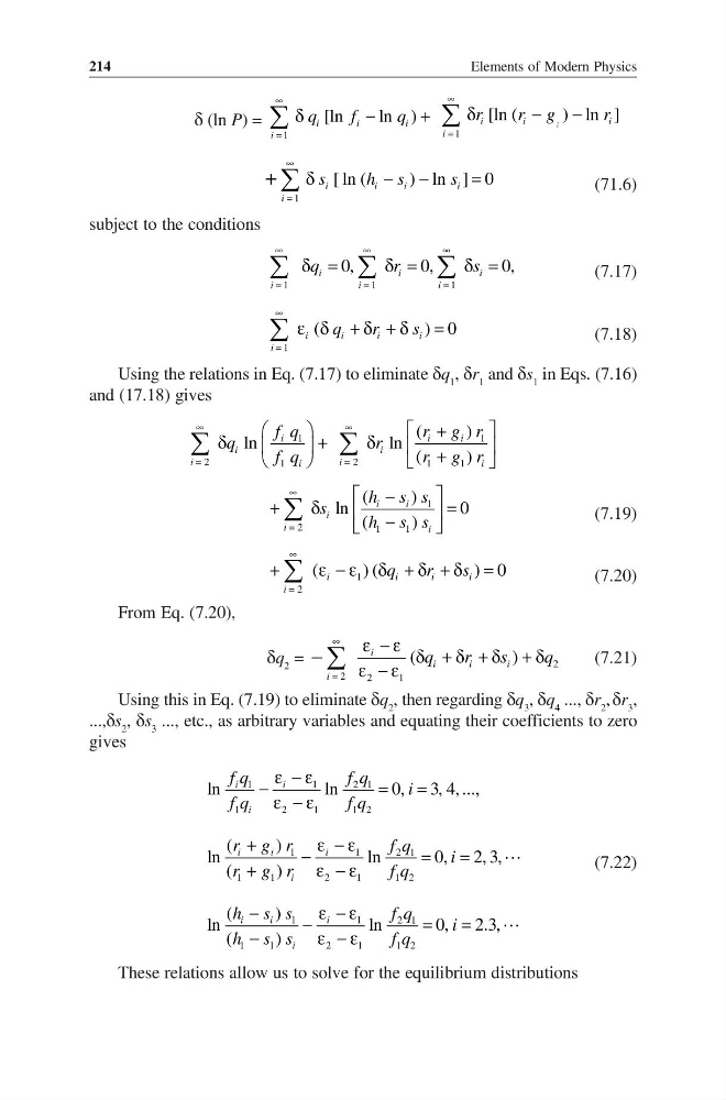
Using the relations in Eq. (7.17) to eliminate δq 1 , δr 1 and δs 1 in Eqs. (7.16)
and (17.18) gives
1
2
1
ln
i
i
i =
i
f q
q
f q
∞
δ
+
∑
1
2
1
1
(
)
ln (
)
i
i
i
i =
i
r g r
r
r g r
∞
+
δ
+
∑
1
2
1
1
(
)
ln
0
(
)
i
i
i
i =
i
h s s
s
h s s
∞
−
+
δ
=
−
∑
(7.19)
1
2
(
)(
) 0
i
i
i
i
i =
q
r
s
∞
+
ε −ε δ +δ +δ =
∑
(7.20)
From Eq. (7.20),
δq 2 =
2
2
2
1
(
)
–
i
i
i
i
i
q
r
s
q
∞
=
ε − ε δ + δ + δ + δ
ε − ε
∑
(7.21)
Using this in Eq. (7.19) to eliminate δq 2 , then regarding δq 3 , δq 4 ..., δr 2 , δr 3 ,
...,δs 2 , δs 3 ..., etc., as arbitrary variables and equating their coefficients to zero
gives
1
1
2 1
1
2
1
1 2
ln
ln
0, 3, 4, ...,
i
i
i
f q
f q
i
f q
f q
ε − ε
−
=
=
ε − ε
1
1
2 1
1
1
2
1
1 2
(
)
ln
ln
0, 2, 3,
(
)
i
i
i
i
r g r
f q
i
r g r
f q
+
ε −ε
−
=
=
+
ε −ε
(7.22)
1
1
2 1
1
1
2
1
1 2
(
)
ln
ln
0, 2.3,
(
)
i
i
i
i
h s s
f q
i
h s s
f q
−
ε −ε
−
=
=
−
ε −ε
These relations allow us to solve for the equilibrium distributions
214
δ (ln P) =
1
[ln
ln )
i
i
i
i
q
f
q
∞
=
δ
−
+
∑
1
[ln (
) ln ]
i
i
i
i
i
r
r g
r
∞
=
δ
−
−
∑
1
[ ln (
) ln ] 0
+
i
i
i
i
i =
s
h s
s
∞
δ
− −
=
∑
(71.6)
subject to the conditions
1
1
1
0,
0,
0,
i
i
i
i =
i =
i =
q
r
s
∞
∞
∞
δ =
δ =
δ =
∑
∑
∑
(7.17)
1
(
) 0
i
i
i
i
i =
q
r
s
∞
ε δ + δ + δ =
∑
(7.18)
Using the relations in Eq. (7.17) to eliminate δq 1 , δr 1 and δs 1 in Eqs. (7.16)
and (17.18) gives
1
2
1
ln
i
i
i =
i
f q
q
f q
∞
δ
+
∑
1
2
1
1
(
)
ln (
)
i
i
i
i =
i
r g r
r
r g r
∞
+
δ
+
∑
1
2
1
1
(
)
ln
0
(
)
i
i
i
i =
i
h s s
s
h s s
∞
−
+
δ
=
−
∑
(7.19)
1
2
(
)(
) 0
i
i
i
i
i =
q
r
s
∞
+
ε −ε δ +δ +δ =
∑
(7.20)
From Eq. (7.20),
δq 2 =
2
2
2
1
(
)
–
i
i
i
i
i
q
r
s
q
∞
=
ε − ε δ + δ + δ + δ
ε − ε
∑
(7.21)
Using this in Eq. (7.19) to eliminate δq 2 , then regarding δq 3 , δq 4 ..., δr 2 , δr 3 ,
...,δs 2 , δs 3 ..., etc., as arbitrary variables and equating their coefficients to zero
gives
1
1
2 1
1
2
1
1 2
ln
ln
0, 3, 4, ...,
i
i
i
f q
f q
i
f q
f q
ε − ε
−
=
=
ε − ε
1
1
2 1
1
1
2
1
1 2
(
)
ln
ln
0, 2, 3,
(
)
i
i
i
i
r g r
f q
i
r g r
f q
+
ε −ε
−
=
=
+
ε −ε
(7.22)
1
1
2 1
1
1
2
1
1 2
(
)
ln
ln
0, 2.3,
(
)
i
i
i
i
h s s
f q
i
h s s
f q
−
ε −ε
−
=
=
−
ε −ε
These relations allow us to solve for the equilibrium distributions