

Interaction with External Fields
203
Measurement of Lifetimes
The measurement of lifetimes of excited atoms and molecules, being of the
order of 10
–8
s, is difficult. A few techniques of measuring short lifetimes are
discussed here.
The lifetimes can be obtained by measuring the intensity of radiation from
a collection of excited atoms, as a function of time. A voltage pulse is used to
excite the atoms by electron bombardment. The pulse starts the multi-channel
analyser in which channel n is active during the time nδ to (n + 1)δ, δ being a
time interval short compared with the lifetime τ of the atoms. The channel
records the pulses produced by the photoelectrons generated by the radiation
emitted. The pulse intensity is proportional to the number of excited atoms, and
hence its time dependence allows us to calculate the lifetime [from Eq. (6.76)].
One of the difficulties is that the population in the decaying state may be
continuously replenished by the particles in a higher excited state decaying to
the lower excited state under consideration.
In another method for measuring lifetimes of excited ions, called the beamfoil technique, fast moving ions (accelerated by a potential difference) are excited
by passing them through a thin foil. The intensity of radiation emitted as a
function of the distance these excited ions travel, gives us information about
the number of excited states as a function of time, and hence allows us to calculate
the lifetime τ [from Eq. (6.76)].
An indirect method of calculating the natural lifetime is to measure the
linewidth of the level, and use the relation τ = 1/∆ω (essentially the uncertainty
relation) to deduce the lifetime of the state. In this method, the Doppler linewidth
and the collision linewidth (collisions affect the lifetime of a state), must be
taken into account in isolating the natural linewidth from the total observed
linewidth (∆ω used in the uncertainty relation is the natural line width).
6.8 EXAMPLES
The discussion in this chapter is now supplemented with some technical details
and examples.
Example 1
Here, the proof of the important theorem stated in Sec. 6.2 is outlined. To prove
the equality in Eq. (6.8), the z-axis is taken along the direction under
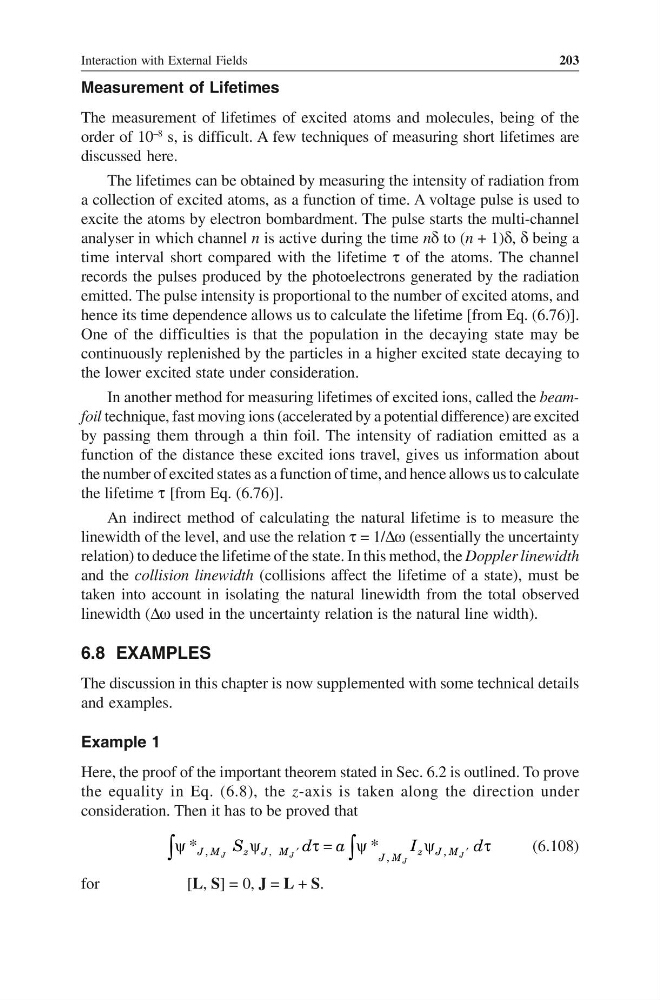
consideration. Then it has to be proved that
,
,
,
*
*
J
J
J
J
J M
z J M
z J M
J M
S
d
a
I
d
,
′
′
ψ
ψ
τ=
ψ
ψ
τ
∫
∫
(6.108)
for
[L, S] = 0, J = L + S.
203
Measurement of Lifetimes
The measurement of lifetimes of excited atoms and molecules, being of the
order of 10
–8
s, is difficult. A few techniques of measuring short lifetimes are
discussed here.
The lifetimes can be obtained by measuring the intensity of radiation from
a collection of excited atoms, as a function of time. A voltage pulse is used to
excite the atoms by electron bombardment. The pulse starts the multi-channel
analyser in which channel n is active during the time nδ to (n + 1)δ, δ being a
time interval short compared with the lifetime τ of the atoms. The channel
records the pulses produced by the photoelectrons generated by the radiation
emitted. The pulse intensity is proportional to the number of excited atoms, and
hence its time dependence allows us to calculate the lifetime [from Eq. (6.76)].
One of the difficulties is that the population in the decaying state may be
continuously replenished by the particles in a higher excited state decaying to
the lower excited state under consideration.
In another method for measuring lifetimes of excited ions, called the beamfoil technique, fast moving ions (accelerated by a potential difference) are excited
by passing them through a thin foil. The intensity of radiation emitted as a
function of the distance these excited ions travel, gives us information about
the number of excited states as a function of time, and hence allows us to calculate
the lifetime τ [from Eq. (6.76)].
An indirect method of calculating the natural lifetime is to measure the
linewidth of the level, and use the relation τ = 1/∆ω (essentially the uncertainty
relation) to deduce the lifetime of the state. In this method, the Doppler linewidth
and the collision linewidth (collisions affect the lifetime of a state), must be
taken into account in isolating the natural linewidth from the total observed
linewidth (∆ω used in the uncertainty relation is the natural line width).
6.8 EXAMPLES
The discussion in this chapter is now supplemented with some technical details
and examples.
Example 1
Here, the proof of the important theorem stated in Sec. 6.2 is outlined. To prove
the equality in Eq. (6.8), the z-axis is taken along the direction under
consideration. Then it has to be proved that
,
,
,
*
*
J
J
J
J
J M
z J M
z J M
J M
S
d
a
I
d
,
′
′
ψ
ψ
τ=
ψ
ψ
τ
∫
∫
(6.108)
for
[L, S] = 0, J = L + S.