

The One-Electron Atom
103
2
2
2
2
2
( )
( )
2
2
∂
∂
−
φ +
φ
∂
∂
r
r
r
r
r
m r
m r
L
r
r
2
0
( )
4
−
φ
πε
Ze
r
r = Eφ (r)
(4.8)
with the angular nominatum term L
2
given by Eq. (3.137).
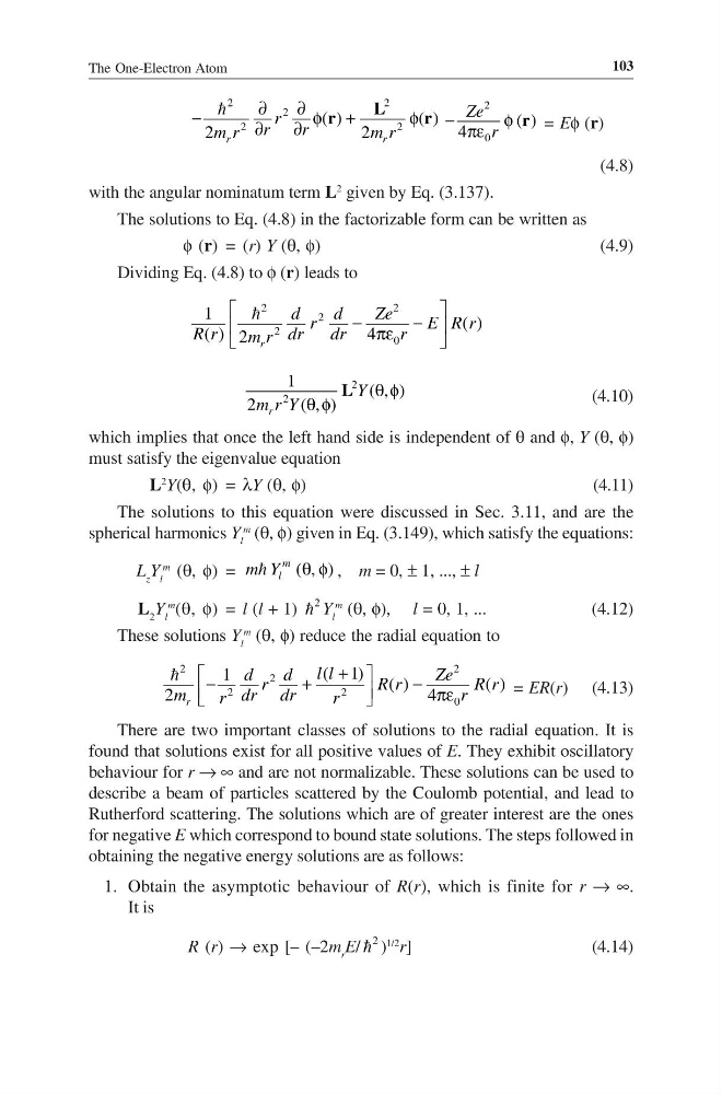
The solutions to Eq. (4.8) in the factorizable form can be written as
φ (r) = (r) Y (θ, φ)
(4.9)
Dividing Eq. (4.8) to φ (r) leads to
2
2
2
2
0
1
( )
( )
4
2 r
d
d
Ze
r
E Rr
R r
dr
dr
r
m r
−
−
πε
2
2
1
( , )
2
( , )
θ φ
θ φ
r
Y
m r Y
L
(4.10)
which implies that once the left hand side is independent of θ and φ, Y (θ, φ)
must satisfy the eigenvalue equation
L
2
Y(θ, φ) = λY (θ, φ)
(4.11)
The solutions to this equation were discussed in Sec. 3.11, and are the
spherical harmonics Y l
m
(θ, φ) given in Eq. (3.149), which satisfy the equations:
L z Y l
m
(θ, φ) =
( , )
m
l
m Y θ φ
, m = 0, ± 1, ..., ± l
L 2 Y l
m
(θ, φ) = l (l + 1)
2
Y l
m
(θ, φ), l = 0, 1, ...
(4.12)
These solutions Y l
m
(θ, φ) reduce the radial equation to
2
2
2
2
2
0
( 1)
1
( )
( )
2
4
r
l l
d
d
Ze
r
Rr
Rr
m
dr dr
r
r
r
+
−
+
−
πε
= ER(r) (4.13)
There are two important classes of solutions to the radial equation. It is
found that solutions exist for all positive values of E. They exhibit oscillatory
behaviour for r → ∞ and are not normalizable. These solutions can be used to
describe a beam of particles scattered by the Coulomb potential, and lead to
Rutherford scattering. The solutions which are of greater interest are the ones
for negative E which correspond to bound state solutions. The steps followed in
obtaining the negative energy solutions are as follows:
1. Obtain the asymptotic behaviour of R(r), which is finite for r → ∞.
It is
R (r) → exp [– (–2m r E/
2
)
1/2
r]
(4.14)
103
2
2
2
2
2
( )
( )
2
2
∂
∂
−
φ +
φ
∂
∂
r
r
r
r
r
m r
m r
L
r
r
2
0
( )
4
−
φ
πε
Ze
r
r = Eφ (r)
(4.8)
with the angular nominatum term L
2
given by Eq. (3.137).
The solutions to Eq. (4.8) in the factorizable form can be written as
φ (r) = (r) Y (θ, φ)
(4.9)
Dividing Eq. (4.8) to φ (r) leads to
2
2
2
2
0
1
( )
( )
4
2 r
d
d
Ze
r
E Rr
R r
dr
dr
r
m r
−
−
πε
2
2
1
( , )
2
( , )
θ φ
θ φ
r
Y
m r Y
L
(4.10)
which implies that once the left hand side is independent of θ and φ, Y (θ, φ)
must satisfy the eigenvalue equation
L
2
Y(θ, φ) = λY (θ, φ)
(4.11)
The solutions to this equation were discussed in Sec. 3.11, and are the
spherical harmonics Y l
m
(θ, φ) given in Eq. (3.149), which satisfy the equations:
L z Y l
m
(θ, φ) =
( , )
m
l
m Y θ φ
, m = 0, ± 1, ..., ± l
L 2 Y l
m
(θ, φ) = l (l + 1)
2
Y l
m
(θ, φ), l = 0, 1, ...
(4.12)
These solutions Y l
m
(θ, φ) reduce the radial equation to
2
2
2
2
2
0
( 1)
1
( )
( )
2
4
r
l l
d
d
Ze
r
Rr
Rr
m
dr dr
r
r
r
+
−
+
−
πε
= ER(r) (4.13)
There are two important classes of solutions to the radial equation. It is
found that solutions exist for all positive values of E. They exhibit oscillatory
behaviour for r → ∞ and are not normalizable. These solutions can be used to
describe a beam of particles scattered by the Coulomb potential, and lead to
Rutherford scattering. The solutions which are of greater interest are the ones
for negative E which correspond to bound state solutions. The steps followed in
obtaining the negative energy solutions are as follows:
1. Obtain the asymptotic behaviour of R(r), which is finite for r → ∞.
It is
R (r) → exp [– (–2m r E/
2
)
1/2
r]
(4.14)