

4.1 Newton Model
85
10
−3 10
−2 10
−1 10
0 10
1 10
2 10
3
10
−6
10
−3
10
0
10
3
10
6
ω
E
η = 10
2
, 10
1
, 10
0
, 10
−1
, 10
−2
ωη
10
−3 10
−2 10
−1 10
0 10
1 10
2 10
3
10
−6
10
−3
10
0
10
3
10
6
ω
C
η = 10
2
, 10
1
, 10
0
, 10
−1
, 10
−2
1
ωη
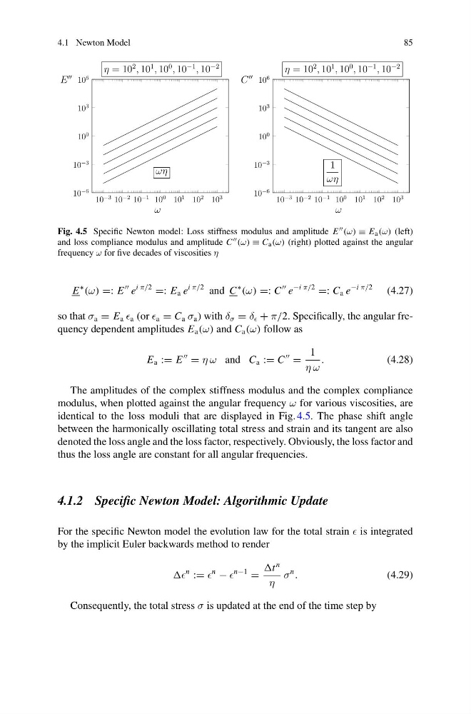
Fig. 4.5 Specific Newton model: Loss stiffness modulus and amplitude E (ω) ≡ E a (ω) (left)
and loss compliance modulus and amplitude C (ω) ≡ C a (ω) (right) plotted against the angular
frequency ω for five decades of viscosities η
E
∗
(ω) =: E
e
i π/2
=: E a e
i π/2 and C
∗
(ω) =: C
e
−i π/2
=: C a e
−i π/2
(4.27)
so that σ a = E a a (or a = C a σ a ) with δ σ = δ + π/2. Specifically, the angular frequency dependent amplitudes E a (ω) and C a (ω) follow as
E a := E
= η ω and C a := C
=
1
η ω
.
(4.28)
The amplitudes of the complex stiffness modulus and the complex compliance
modulus, when plotted against the angular frequency ω for various viscosities, are
identical to the loss moduli that are displayed in Fig. 4.5. The phase shift angle
between the harmonically oscillating total stress and strain and its tangent are also
denoted the loss angle and the loss factor, respectively. Obviously, the loss factor and
thus the loss angle are constant for all angular frequencies.
4.1.2 Specific Newton Model: Algorithmic Update
For the specific Newton model the evolution law for the total strain is integrated
by the implicit Euler backwards method to render
n
:=
n
−
n−1
=
n
η
σ
n
.
(4.29)
Consequently, the total stress σ is updated at the end of the time step by
85
10
−3 10
−2 10
−1 10
0 10
1 10
2 10
3
10
−6
10
−3
10
0
10
3
10
6
ω
E
η = 10
2
, 10
1
, 10
0
, 10
−1
, 10
−2
ωη
10
−3 10
−2 10
−1 10
0 10
1 10
2 10
3
10
−6
10
−3
10
0
10
3
10
6
ω
C
η = 10
2
, 10
1
, 10
0
, 10
−1
, 10
−2
1
ωη
Fig. 4.5 Specific Newton model: Loss stiffness modulus and amplitude E (ω) ≡ E a (ω) (left)
and loss compliance modulus and amplitude C (ω) ≡ C a (ω) (right) plotted against the angular
frequency ω for five decades of viscosities η
E
∗
(ω) =: E
e
i π/2
=: E a e
i π/2 and C
∗
(ω) =: C
e
−i π/2
=: C a e
−i π/2
(4.27)
so that σ a = E a a (or a = C a σ a ) with δ σ = δ + π/2. Specifically, the angular frequency dependent amplitudes E a (ω) and C a (ω) follow as
E a := E
= η ω and C a := C
=
1
η ω
.
(4.28)
The amplitudes of the complex stiffness modulus and the complex compliance
modulus, when plotted against the angular frequency ω for various viscosities, are
identical to the loss moduli that are displayed in Fig. 4.5. The phase shift angle
between the harmonically oscillating total stress and strain and its tangent are also
denoted the loss angle and the loss factor, respectively. Obviously, the loss factor and
thus the loss angle are constant for all angular frequencies.
4.1.2 Specific Newton Model: Algorithmic Update
For the specific Newton model the evolution law for the total strain is integrated
by the implicit Euler backwards method to render
n
:=
n
−
n−1
=
n
η
σ
n
.
(4.29)
Consequently, the total stress σ is updated at the end of the time step by