

84
4 Visco-Elasticity
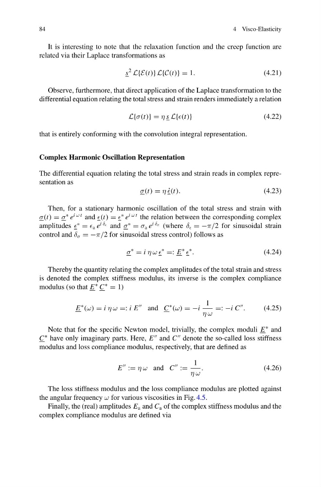
It is interesting to note that the relaxation function and the creep function are
related via their Laplace transformations as
s
2
L{E(t)} L{C(t)} = 1.
(4.21)
Observe, furthermore, that direct application of the Laplace transformation to the
differential equation relating the total stress and strain renders immediately a relation
L{σ(t)} = η s L{(t)}
(4.22)
that is entirely conforming with the convolution integral representation.
Complex Harmonic Oscillation Representation
The differential equation relating the total stress and strain reads in complex representation as
σ(t) = η ˙
(t).
(4.23)
Then, for a stationary harmonic oscillation of the total stress and strain with
σ(t) = σ
∗ e
i ω t and (t) =
∗ e
i ω t the relation between the corresponding complex
amplitudes
∗
= a e
i δ and σ
∗
= σ a e
i δ σ (where δ = −π/2 for sinusoidal strain
control and δ σ = −π/2 for sinusoidal stress control) follows as
σ
∗
= i η ω ω
∗
=: E
∗
∗
.
(4.24)
Thereby the quantity relating the complex amplitudes of the total strain and stress
is denoted the complex stiffness modulus, its inverse is the complex compliance
modulus (so that E
∗ C
∗
= 1)
E
∗
(ω) = i η ω =: i E
and C
∗
(ω) = −i
1
η ω
=: −i C
.
(4.25)
Note that for the specific Newton model, trivially, the complex moduli E
∗ and
C
∗ have only imaginary parts. Here, E
and C
denote the so-called loss stiffness
modulus and loss compliance modulus, respectively, that are defined as
E
:= η ω and C
:=
1
η ω
.
(4.26)
The loss stiffness modulus and the loss compliance modulus are plotted against
the angular frequency ω for various viscosities in Fig. 4.5.
Finally, the (real) amplitudes E a and C a of the complex stiffness modulus and the
complex compliance modulus are defined via
4 Visco-Elasticity
It is interesting to note that the relaxation function and the creep function are
related via their Laplace transformations as
s
2
L{E(t)} L{C(t)} = 1.
(4.21)
Observe, furthermore, that direct application of the Laplace transformation to the
differential equation relating the total stress and strain renders immediately a relation
L{σ(t)} = η s L{(t)}
(4.22)
that is entirely conforming with the convolution integral representation.
Complex Harmonic Oscillation Representation
The differential equation relating the total stress and strain reads in complex representation as
σ(t) = η ˙
(t).
(4.23)
Then, for a stationary harmonic oscillation of the total stress and strain with
σ(t) = σ
∗ e
i ω t and (t) =
∗ e
i ω t the relation between the corresponding complex
amplitudes
∗
= a e
i δ and σ
∗
= σ a e
i δ σ (where δ = −π/2 for sinusoidal strain
control and δ σ = −π/2 for sinusoidal stress control) follows as
σ
∗
= i η ω ω
∗
=: E
∗
∗
.
(4.24)
Thereby the quantity relating the complex amplitudes of the total strain and stress
is denoted the complex stiffness modulus, its inverse is the complex compliance
modulus (so that E
∗ C
∗
= 1)
E
∗
(ω) = i η ω =: i E
and C
∗
(ω) = −i
1
η ω
=: −i C
.
(4.25)
Note that for the specific Newton model, trivially, the complex moduli E
∗ and
C
∗ have only imaginary parts. Here, E
and C
denote the so-called loss stiffness
modulus and loss compliance modulus, respectively, that are defined as
E
:= η ω and C
:=
1
η ω
.
(4.26)
The loss stiffness modulus and the loss compliance modulus are plotted against
the angular frequency ω for various viscosities in Fig. 4.5.
Finally, the (real) amplitudes E a and C a of the complex stiffness modulus and the
complex compliance modulus are defined via