

3.1 Hooke Model
75
ψ ( = max
σ
{σ σ − ψ
∗
(σ)},
(3.30a)
ψ
∗
(σ) = max
{σ σ − ψ (
(3.30b)
The stationarity conditions corresponding to Eqs. 3.30a and 3.30b are the constitutive
relations
= ∂ σ ψ
∗
(σ),
(3.31a)
σ( = ∂ ψ ( ).
(3.31b)
Obviously, the relations in Eqs. 3.31a and 3.31b determine entirely the energetic
behaviour of the generic Hooke model, thus the formulation is completed at this
stage.
It is finally emphasized that due to the entirely energetic character of the generic
Hooke model the dissipation inequality d ≤ 0 degenerates to the strict equality d = 0.
The generic Hooke model is summarized in Table 3.3.
Table 3.3 Summary of the generic Hooke model
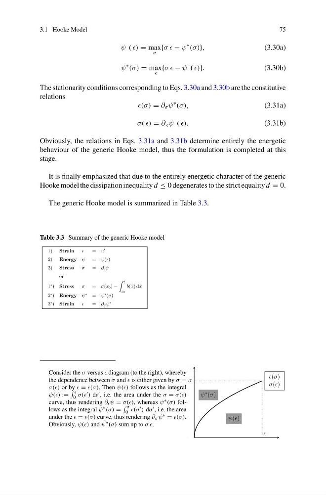
Consider the σ versus diagram (to the right), whereby
the dependence between σ and is either given by σ =
σ( or by = Then ψ( follows as the integral
ψ( :=
0 σ( ) d , i.e. the area under the σ = σ(
curve, thus rendering ∂ ψ = σ( whereas ψ ∗ (σ) follows as the integral ψ ∗ (σ) =
σ
0 ) dσ , i.e. the area
under the = curve, thus rendering ∂ σ ψ ∗ =
Obviously, ψ( and ψ ∗ (σ) sum up to σ σ.
σ
(σ)
σ( )
ψ
∗ (σ)
ψ( )
75
ψ ( = max
σ
{σ σ − ψ
∗
(σ)},
(3.30a)
ψ
∗
(σ) = max
{σ σ − ψ (
(3.30b)
The stationarity conditions corresponding to Eqs. 3.30a and 3.30b are the constitutive
relations
= ∂ σ ψ
∗
(σ),
(3.31a)
σ( = ∂ ψ ( ).
(3.31b)
Obviously, the relations in Eqs. 3.31a and 3.31b determine entirely the energetic
behaviour of the generic Hooke model, thus the formulation is completed at this
stage.
It is finally emphasized that due to the entirely energetic character of the generic
Hooke model the dissipation inequality d ≤ 0 degenerates to the strict equality d = 0.
The generic Hooke model is summarized in Table 3.3.
Table 3.3 Summary of the generic Hooke model
Consider the σ versus diagram (to the right), whereby
the dependence between σ and is either given by σ =
σ( or by = Then ψ( follows as the integral
ψ( :=
0 σ( ) d , i.e. the area under the σ = σ(
curve, thus rendering ∂ ψ = σ( whereas ψ ∗ (σ) follows as the integral ψ ∗ (σ) =
σ
0 ) dσ , i.e. the area
under the = curve, thus rendering ∂ σ ψ ∗ =
Obviously, ψ( and ψ ∗ (σ) sum up to σ σ.
σ
(σ)
σ( )
ψ
∗ (σ)
ψ( )