

60
2 Preliminaries
Thus, the Lagrange multiplier is proportional to the constraint violation, whereby the
proportionality factor ε is denoted the perturbation or rather the penalty parameter.
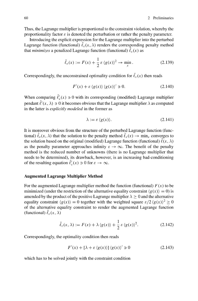
Introducing the explicit expression for the Lagrange multiplier into the perturbed
Lagrange function (functional) ˆ
ε (x, λ) renders the corresponding penalty method
that minimizes a penalized Lagrange function (functional) ˜
ε (x) as
˜
ε (x) := F(x) +
1
2
ε g(x)
2
→ min
x
.
(2.139)
Correspondingly, the unconstrained optimality condition for ˜
ε (x) then reads
F
(x) + ε g(x) g(x)
0.
(2.140)
When comparing ˜
ε (x) 0 with its corresponding (modified) Lagrange multiplier
pendant ˆ
(x, λ) 0 it becomes obvious that the Lagrange multiplier λ as computed
in the latter is explicitly modeled in the former as
λ := ε g(x).
(2.141)
It is moreover obvious from the structure of the perturbed Lagrange function (functional) ˆ
ε (x, λ) that the solution to the penalty method ˜
ε (x) → min x converges to
the solution based on the original (modified) Lagrange function (functional) ˆ
(x, λ)
as the penalty parameter approaches infinity ε → ∞. The benefit of the penalty
method is the reduced number of unknowns (there is no Lagrange multiplier that
needs to be determined), its drawback, however, is an increasing bad-conditioning
of the resulting equation ˜
ε (x) 0 for ε → ∞.
Augmented Lagrange Multiplier Method
For the augmented Lagrange multiplier method the function (functional) F(x) to be
minimized (under the restriction of the alternative equality constraint g(x) = 0) is
amended by the product of the positive Lagrange multiplier λ ≥ 0 and the alternative
equality constraint g(x) = 0 together with the weighted square ε/2 g(x)
2
≥ 0
of the alternative equality constraint to render the augmented Lagrange function
(functional) ˇ
ε (x, λ)
ˇ
ε (x, λ) := F(x) + λ g(x) +
1
2
ε g(x)
2
.
(2.142)
Correspondingly, the optimality condition then reads
F
(x) + [λ + ε g(x)] g(x)
0
(2.143)
which has to be solved jointly with the constraint condition
2 Preliminaries
Thus, the Lagrange multiplier is proportional to the constraint violation, whereby the
proportionality factor ε is denoted the perturbation or rather the penalty parameter.
Introducing the explicit expression for the Lagrange multiplier into the perturbed
Lagrange function (functional) ˆ
ε (x, λ) renders the corresponding penalty method
that minimizes a penalized Lagrange function (functional) ˜
ε (x) as
˜
ε (x) := F(x) +
1
2
ε g(x)
2
→ min
x
.
(2.139)
Correspondingly, the unconstrained optimality condition for ˜
ε (x) then reads
F
(x) + ε g(x) g(x)
0.
(2.140)
When comparing ˜
ε (x) 0 with its corresponding (modified) Lagrange multiplier
pendant ˆ
(x, λ) 0 it becomes obvious that the Lagrange multiplier λ as computed
in the latter is explicitly modeled in the former as
λ := ε g(x).
(2.141)
It is moreover obvious from the structure of the perturbed Lagrange function (functional) ˆ
ε (x, λ) that the solution to the penalty method ˜
ε (x) → min x converges to
the solution based on the original (modified) Lagrange function (functional) ˆ
(x, λ)
as the penalty parameter approaches infinity ε → ∞. The benefit of the penalty
method is the reduced number of unknowns (there is no Lagrange multiplier that
needs to be determined), its drawback, however, is an increasing bad-conditioning
of the resulting equation ˜
ε (x) 0 for ε → ∞.
Augmented Lagrange Multiplier Method
For the augmented Lagrange multiplier method the function (functional) F(x) to be
minimized (under the restriction of the alternative equality constraint g(x) = 0) is
amended by the product of the positive Lagrange multiplier λ ≥ 0 and the alternative
equality constraint g(x) = 0 together with the weighted square ε/2 g(x)
2
≥ 0
of the alternative equality constraint to render the augmented Lagrange function
(functional) ˇ
ε (x, λ)
ˇ
ε (x, λ) := F(x) + λ g(x) +
1
2
ε g(x)
2
.
(2.142)
Correspondingly, the optimality condition then reads
F
(x) + [λ + ε g(x)] g(x)
0
(2.143)
which has to be solved jointly with the constraint condition