

2.2 Computational Tools
45
Thus an iterative update for the global unknowns collected in u follows as the solution
of a linear algebraic equation system in terms of the global residual and the global
tangent stiffness matrix
u ⇐ u + du with du = k
−1 r.
(2.75)
Subsequently, the residual has to be re-evaluated with the updated estimate for u and
the iteration proceeds until convergence with |r| → 0 is achieved. The quadratic convergence of the Newton iteration (in the vicinity of the solution) depends crucially on
the correct determination of k (and the smoothness of the global force-displacement
relation). Observe that no force control is possible as soon as the global tangent
stiffness matrix degenerates with w
t k w ≤ 0 for some w = 0.
2.3 Mathematical Tools
2.3.1 Heaviside Function and Causal Signals
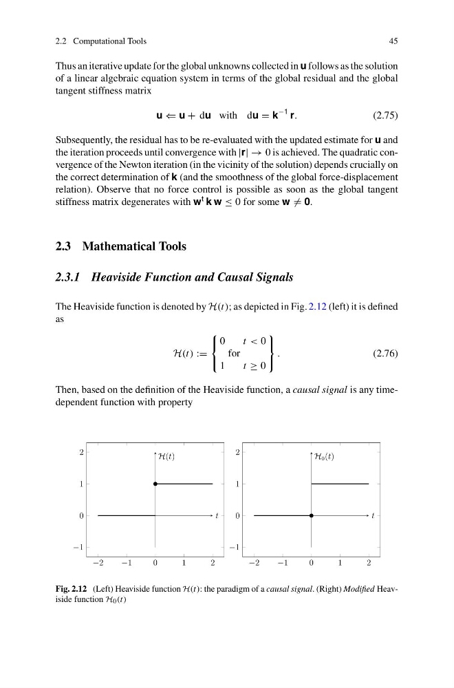
The Heaviside function is denoted by H(t); as depicted in Fig. 2.12 (left) it is defined
as
H(t) :=
⎧
⎨
⎩
0
t < 0
for
1
t ≥ 0
⎫
⎬
⎭
.
(2.76)
Then, based on the definition of the Heaviside function, a causal signal is any timedependent function with property
−2
−1
0
1
2
−1
0
1
2
t
H(t)
−2
−1
0
1
2
−1
0
1
2
t
H 0 (t)
Fig. 2.12 (Left) Heaviside function H(t): the paradigm of a causal signal. (Right) Modified Heaviside function H 0 (t)
45
Thus an iterative update for the global unknowns collected in u follows as the solution
of a linear algebraic equation system in terms of the global residual and the global
tangent stiffness matrix
u ⇐ u + du with du = k
−1 r.
(2.75)
Subsequently, the residual has to be re-evaluated with the updated estimate for u and
the iteration proceeds until convergence with |r| → 0 is achieved. The quadratic convergence of the Newton iteration (in the vicinity of the solution) depends crucially on
the correct determination of k (and the smoothness of the global force-displacement
relation). Observe that no force control is possible as soon as the global tangent
stiffness matrix degenerates with w
t k w ≤ 0 for some w = 0.
2.3 Mathematical Tools
2.3.1 Heaviside Function and Causal Signals
The Heaviside function is denoted by H(t); as depicted in Fig. 2.12 (left) it is defined
as
H(t) :=
⎧
⎨
⎩
0
t < 0
for
1
t ≥ 0
⎫
⎬
⎭
.
(2.76)
Then, based on the definition of the Heaviside function, a causal signal is any timedependent function with property
−2
−1
0
1
2
−1
0
1
2
t
H(t)
−2
−1
0
1
2
−1
0
1
2
t
H 0 (t)
Fig. 2.12 (Left) Heaviside function H(t): the paradigm of a causal signal. (Right) Modified Heaviside function H 0 (t)