

44
2 Preliminaries
u e = a e u with dim a e = n en × n np .
(2.67)
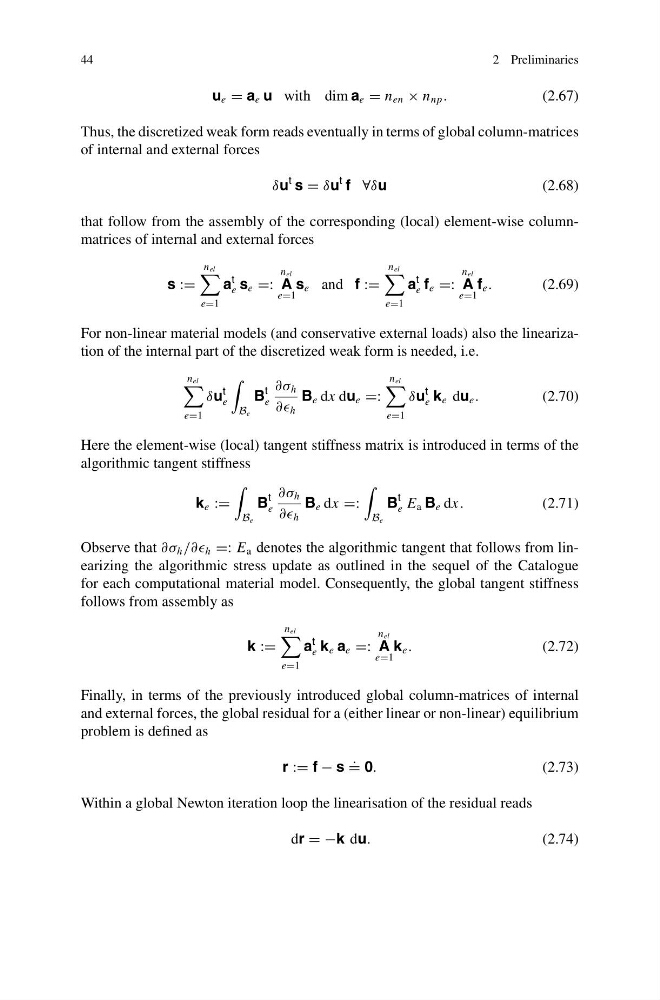
Thus, the discretized weak form reads eventually in terms of global column-matrices
of internal and external forces
δu
t s = δu
t f ∀δu
(2.68)
that follow from the assembly of the corresponding (local) element-wise columnmatrices of internal and external forces
s :=
n el
e=1
a
t
e s e =:
n el
A
e=1
s e and f :=
n el
e=1
a
t
e f e =:
n el
A
e=1
f e .
(2.69)
For non-linear material models (and conservative external loads) also the linearization of the internal part of the discretized weak form is needed, i.e.
n el
e=1
δu
t
e
B e
B
t
e
∂σ h
∂∂ h
B e dx du e =:
n el
e=1
δu
t
e k e du e .
(2.70)
Here the element-wise (local) tangent stiffness matrix is introduced in terms of the
algorithmic tangent stiffness
k e :=
B e
B
t
e
∂σ h
∂∂ h
B e dx =:
B e
B
t
e E a B e dx.
(2.71)
Observe that ∂σ h /∂∂ h =: E a denotes the algorithmic tangent that follows from linearizing the algorithmic stress update as outlined in the sequel of the Catalogue
for each computational material model. Consequently, the global tangent stiffness
follows from assembly as
k :=
n el
e=1
a
t
e k e a e =:
n el
A
e=1
k e .
(2.72)
Finally, in terms of the previously introduced global column-matrices of internal
and external forces, the global residual for a (either linear or non-linear) equilibrium
problem is defined as
r := f − s
.
= 0.
(2.73)
Within a global Newton iteration loop the linearisation of the residual reads
dr = −k du.
(2.74)
2 Preliminaries
u e = a e u with dim a e = n en × n np .
(2.67)
Thus, the discretized weak form reads eventually in terms of global column-matrices
of internal and external forces
δu
t s = δu
t f ∀δu
(2.68)
that follow from the assembly of the corresponding (local) element-wise columnmatrices of internal and external forces
s :=
n el
e=1
a
t
e s e =:
n el
A
e=1
s e and f :=
n el
e=1
a
t
e f e =:
n el
A
e=1
f e .
(2.69)
For non-linear material models (and conservative external loads) also the linearization of the internal part of the discretized weak form is needed, i.e.
n el
e=1
δu
t
e
B e
B
t
e
∂σ h
∂∂ h
B e dx du e =:
n el
e=1
δu
t
e k e du e .
(2.70)
Here the element-wise (local) tangent stiffness matrix is introduced in terms of the
algorithmic tangent stiffness
k e :=
B e
B
t
e
∂σ h
∂∂ h
B e dx =:
B e
B
t
e E a B e dx.
(2.71)
Observe that ∂σ h /∂∂ h =: E a denotes the algorithmic tangent that follows from linearizing the algorithmic stress update as outlined in the sequel of the Catalogue
for each computational material model. Consequently, the global tangent stiffness
follows from assembly as
k :=
n el
e=1
a
t
e k e a e =:
n el
A
e=1
k e .
(2.72)
Finally, in terms of the previously introduced global column-matrices of internal
and external forces, the global residual for a (either linear or non-linear) equilibrium
problem is defined as
r := f − s
.
= 0.
(2.73)
Within a global Newton iteration loop the linearisation of the residual reads
dr = −k du.
(2.74)