

30
2 Preliminaries
Once again, we identify the two (loading) scenarios:
Strain Control: (t) is prescribed, whereby α(t) and σ (t) are solved from the
coupled Eqs. 2.23a and 2.23b.
Stress Control: σ (t) is prescribed, whereby α(t) and (t) are solved from the
coupled Eqs. 2.23a and 2.23b.
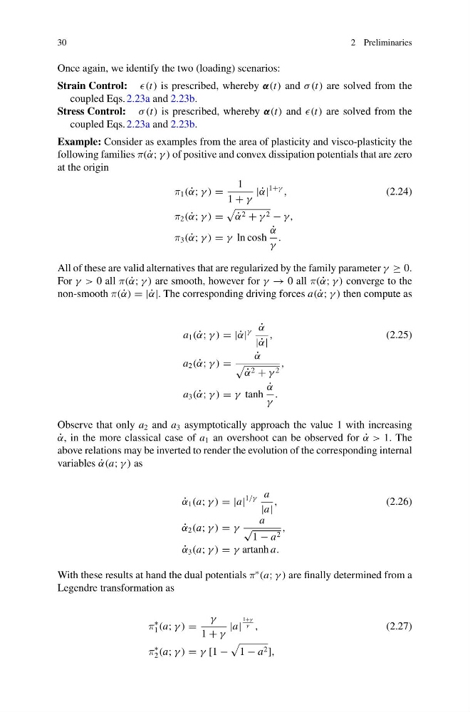
Example: Consider as examples from the area of plasticity and visco-plasticity the
following families π( ˙
α; γ ) of positive and convex dissipation potentials that are zero
at the origin
π 1 ( ˙
α; γ ) =
1
1 + γ
| ˙
α|
1+γ
,
(2.24)
π 2 ( ˙
α; γ ) =
˙
α 2 + γ 2 − γ,
π 3 ( ˙
α; γ ) = γ ln cosh
˙
α
γ
.
All of these are valid alternatives that are regularized by the family parameter γ ≥ 0.
For γ > 0 all π( ˙
α; γ ) are smooth, however for γ → 0 all π( ˙
α; γ ) converge to the
non-smooth π( ˙
α) = | ˙
α|. The corresponding driving forces a( ˙
α; γ ) then compute as
a 1 ( ˙
α; γ ) = | ˙
α|
γ ˙
α
| ˙
α|
,
(2.25)
a 2 ( ˙
α; γ ) =
˙
α
˙
α 2 + γ 2
,
a 3 ( ˙
α; γ ) = γ tanh
˙
α
γ
.
Observe that only a 2 and a 3 asymptotically approach the value 1 with increasing
˙
α, in the more classical case of a 1 an overshoot can be observed for ˙
α > 1. The
above relations may be inverted to render the evolution of the corresponding internal
variables ˙
α(a; γ ) as
˙
α 1 (a; γ ) = |a|
1/γ a
|a|
,
(2.26)
˙
α 2 (a; γ ) = γ
a
√
1 − a 2
,
˙
α 3 (a; γ ) = γ artanh a.
With these results at hand the dual potentials π
∗
(a; γ ) are finally determined from a
Legendre transformation as
π
∗
1 (a; γ ) =
γ
1 + γ
|a|
1+γ
γ ,
(2.27)
π
∗
2 (a; γ ) = γ [1 −
1 − a 2 ],
2 Preliminaries
Once again, we identify the two (loading) scenarios:
Strain Control: (t) is prescribed, whereby α(t) and σ (t) are solved from the
coupled Eqs. 2.23a and 2.23b.
Stress Control: σ (t) is prescribed, whereby α(t) and (t) are solved from the
coupled Eqs. 2.23a and 2.23b.
Example: Consider as examples from the area of plasticity and visco-plasticity the
following families π( ˙
α; γ ) of positive and convex dissipation potentials that are zero
at the origin
π 1 ( ˙
α; γ ) =
1
1 + γ
| ˙
α|
1+γ
,
(2.24)
π 2 ( ˙
α; γ ) =
˙
α 2 + γ 2 − γ,
π 3 ( ˙
α; γ ) = γ ln cosh
˙
α
γ
.
All of these are valid alternatives that are regularized by the family parameter γ ≥ 0.
For γ > 0 all π( ˙
α; γ ) are smooth, however for γ → 0 all π( ˙
α; γ ) converge to the
non-smooth π( ˙
α) = | ˙
α|. The corresponding driving forces a( ˙
α; γ ) then compute as
a 1 ( ˙
α; γ ) = | ˙
α|
γ ˙
α
| ˙
α|
,
(2.25)
a 2 ( ˙
α; γ ) =
˙
α
˙
α 2 + γ 2
,
a 3 ( ˙
α; γ ) = γ tanh
˙
α
γ
.
Observe that only a 2 and a 3 asymptotically approach the value 1 with increasing
˙
α, in the more classical case of a 1 an overshoot can be observed for ˙
α > 1. The
above relations may be inverted to render the evolution of the corresponding internal
variables ˙
α(a; γ ) as
˙
α 1 (a; γ ) = |a|
1/γ a
|a|
,
(2.26)
˙
α 2 (a; γ ) = γ
a
√
1 − a 2
,
˙
α 3 (a; γ ) = γ artanh a.
With these results at hand the dual potentials π
∗
(a; γ ) are finally determined from a
Legendre transformation as
π
∗
1 (a; γ ) =
γ
1 + γ
|a|
1+γ
γ ,
(2.27)
π
∗
2 (a; γ ) = γ [1 −
1 − a 2 ],