

2.1 Modelling Tools
29
π
∗
= π
∗
(σ
, a
)
(2.17)
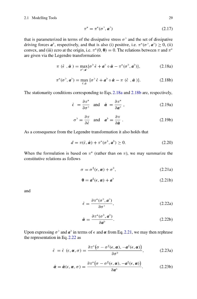
that is parameterized in terms of the dissipative stress σ
and the set of dissipative
driving forces a
, respectively, and that is also (i) positive, i.e. π
∗
(σ
, a
) ≥ 0, (ii)
convex, and (iii) zero at the origin, i.e. π
∗
(0, 0) = 0. The relations between π and π
∗
are given via the Legendre transformations
π (˙ , ˙
α ) = max
σ ,a
{σ
˙
+ a
◦ ˙
α − π
∗
(σ
, a
)},
(2.18a)
π
∗
(σ
, a
) = max
˙
, ˙
α
{σ
˙
+ a
◦ ˙
α − π (˙ , ˙
α )}.
(2.18b)
The stationarity conditions corresponding to Eqs. 2.18a and 2.18b are, respectively,
˙
=
∂π
∗
∂σ and ˙
α =
∂π
∗
∂ a ,
(2.19a)
σ
=
∂π
∂ ˙
and a
=
∂π
∂ ˙
α
.
(2.19b)
As a consequence from the Legendre transformation it also holds that
d = π(˙ , ˙
α) + π
∗
(σ
, a
) ≥ 0.
(2.20)
When the formulation is based on π
∗ (rather than on π), we may summarize the
constitutive relations as follows
σ = σ
((, α) + σ
,
(2.21a)
0 = a
((, α) + a
(2.21b)
and
˙
=
∂π
∗
(σ
, a
)
∂σ
,
(2.22a)
˙
α =
∂π
∗
(σ
, a
)
∂ a
.
(2.22b)
Upon expressing σ
and a
in terms of and α from Eq. 2.21, we may then rephrase
the representation in Eq. 2.22 as
˙
= ˙
((, α, σ ) =
∂π
∗
σ − σ
((, α), −a
((, α)
∂σ
,
(2.23a)
˙
α = ˙
α((, α, σ ) =
∂π
∗
σ − σ
((, α), −a
((, α)
∂ a
.
(2.23b)
29
π
∗
= π
∗
(σ
, a
)
(2.17)
that is parameterized in terms of the dissipative stress σ
and the set of dissipative
driving forces a
, respectively, and that is also (i) positive, i.e. π
∗
(σ
, a
) ≥ 0, (ii)
convex, and (iii) zero at the origin, i.e. π
∗
(0, 0) = 0. The relations between π and π
∗
are given via the Legendre transformations
π (˙ , ˙
α ) = max
σ ,a
{σ
˙
+ a
◦ ˙
α − π
∗
(σ
, a
)},
(2.18a)
π
∗
(σ
, a
) = max
˙
, ˙
α
{σ
˙
+ a
◦ ˙
α − π (˙ , ˙
α )}.
(2.18b)
The stationarity conditions corresponding to Eqs. 2.18a and 2.18b are, respectively,
˙
=
∂π
∗
∂σ and ˙
α =
∂π
∗
∂ a ,
(2.19a)
σ
=
∂π
∂ ˙
and a
=
∂π
∂ ˙
α
.
(2.19b)
As a consequence from the Legendre transformation it also holds that
d = π(˙ , ˙
α) + π
∗
(σ
, a
) ≥ 0.
(2.20)
When the formulation is based on π
∗ (rather than on π), we may summarize the
constitutive relations as follows
σ = σ
((, α) + σ
,
(2.21a)
0 = a
((, α) + a
(2.21b)
and
˙
=
∂π
∗
(σ
, a
)
∂σ
,
(2.22a)
˙
α =
∂π
∗
(σ
, a
)
∂ a
.
(2.22b)
Upon expressing σ
and a
in terms of and α from Eq. 2.21, we may then rephrase
the representation in Eq. 2.22 as
˙
= ˙
((, α, σ ) =
∂π
∗
σ − σ
((, α), −a
((, α)
∂σ
,
(2.23a)
˙
α = ˙
α((, α, σ ) =
∂π
∗
σ − σ
((, α), −a
((, α)
∂ a
.
(2.23b)