

2.1 Modelling Tools
27
uct ◦, norm |α|
2
:= α ◦ α and time derivative defined as ˙
α := { ˙
α 1 , ˙
α 2 , . . .}). Without
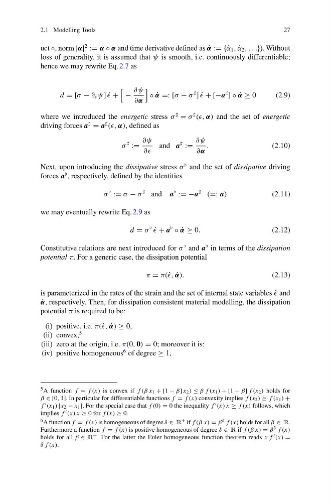
loss of generality, it is assumed that ψ is smooth, i.e. continuously differentiable;
hence we may rewrite Eq. 2.7 as
d = [σ − ∂ ψ] ˙
+
−
∂ψ
∂α
◦ ˙
α =: [σ − σ
] ˙
+ [−a
] ◦ ˙
α ≥ 0
(2.9)
where we introduced the energetic stress σ
= σ
((, α) and the set of energetic
driving forces a
= a
((, α), defined as
σ
:=
∂ψ
∂∂
and a
:=
∂ψ
∂α
.
(2.10)
Next, upon introducing the dissipative stress σ
and the set of dissipative driving
forces a
, respectively, defined by the identities
σ
:= σ − σ
and a
:= −a
(=: a)
(2.11)
we may eventually rewrite Eq. 2.9 as
d = σ
˙
+ a
◦ ˙
α ≥ 0.
(2.12)
Constitutive relations are next introduced for σ
and a
in terms of the dissipation
potential π. For a generic case, the dissipation potential
π = π(˙ , ˙
α).
(2.13)
is parameterized in the rates of the strain and the set of internal state variables ˙
and
˙
α, respectively. Then, for dissipation consistent material modelling, the dissipation
potential π is required to be:
(i) positive, i.e. π(˙ , ˙
α) ≥ 0,
(ii) convex,
5
(iii) zero at the origin, i.e. π(0, 0) = 0; moreover it is:
(iv) positive homogeneous
6 of degree ≥ 1,
5 A function f = f (x) is convex if f (β x 1 + [1 − β] x 2 ) ≤ β f (x 1 ) + [1 − β] f (x 2 ) holds for
β ∈ [0, 1]. In particular for differentiable functions f = f (x) convexity implies f (x 2 ) ≥ f (x 1 ) +
f (x 1 ) [x 2 − x 1 ]. For the special case that f (0) = 0 the inequality f (x) x ≥ f (x) follows, which
implies f (x) x ≥ 0 for f (x) ≥ 0.
6 A function f = f (x) is homogeneous of degree δ ∈ R + if f (β x) = β δ f (x) holds for all β ∈ R.
Furthermore a function f = f (x) is positive homogeneous of degree δ ∈ R if f (β x) = β δ f (x)
holds for all β ∈ R + . For the latter the Euler homogeneous function theorem reads x f (x) =
δ f (x).
27
uct ◦, norm |α|
2
:= α ◦ α and time derivative defined as ˙
α := { ˙
α 1 , ˙
α 2 , . . .}). Without
loss of generality, it is assumed that ψ is smooth, i.e. continuously differentiable;
hence we may rewrite Eq. 2.7 as
d = [σ − ∂ ψ] ˙
+
−
∂ψ
∂α
◦ ˙
α =: [σ − σ
] ˙
+ [−a
] ◦ ˙
α ≥ 0
(2.9)
where we introduced the energetic stress σ
= σ
((, α) and the set of energetic
driving forces a
= a
((, α), defined as
σ
:=
∂ψ
∂∂
and a
:=
∂ψ
∂α
.
(2.10)
Next, upon introducing the dissipative stress σ
and the set of dissipative driving
forces a
, respectively, defined by the identities
σ
:= σ − σ
and a
:= −a
(=: a)
(2.11)
we may eventually rewrite Eq. 2.9 as
d = σ
˙
+ a
◦ ˙
α ≥ 0.
(2.12)
Constitutive relations are next introduced for σ
and a
in terms of the dissipation
potential π. For a generic case, the dissipation potential
π = π(˙ , ˙
α).
(2.13)
is parameterized in the rates of the strain and the set of internal state variables ˙
and
˙
α, respectively. Then, for dissipation consistent material modelling, the dissipation
potential π is required to be:
(i) positive, i.e. π(˙ , ˙
α) ≥ 0,
(ii) convex,
5
(iii) zero at the origin, i.e. π(0, 0) = 0; moreover it is:
(iv) positive homogeneous
6 of degree ≥ 1,
5 A function f = f (x) is convex if f (β x 1 + [1 − β] x 2 ) ≤ β f (x 1 ) + [1 − β] f (x 2 ) holds for
β ∈ [0, 1]. In particular for differentiable functions f = f (x) convexity implies f (x 2 ) ≥ f (x 1 ) +
f (x 1 ) [x 2 − x 1 ]. For the special case that f (0) = 0 the inequality f (x) x ≥ f (x) follows, which
implies f (x) x ≥ 0 for f (x) ≥ 0.
6 A function f = f (x) is homogeneous of degree δ ∈ R + if f (β x) = β δ f (x) holds for all β ∈ R.
Furthermore a function f = f (x) is positive homogeneous of degree δ ∈ R if f (β x) = β δ f (x)
holds for all β ∈ R + . For the latter the Euler homogeneous function theorem reads x f (x) =
δ f (x).