

6.2 Perzyna Model
317
whereby ˜
1/η is a penalized Lagrange functional incorporating the admissibility
constraint |σ vp | ≤ σ y penalized by the penalty parameter 1/η. In accordance with
Eq. 6.83 the stationarity condition of this unconstrained optimization problem then
reads
˙
vp (σ vp ) =
|σ vp | − σ y
η
σ vp
|σ vp |
.
(6.89)
Finally, the visco-plastic strain arc-length, denoted κ, may conveniently be introduced as a measure of the accumulated visco-plastic deformation, i.e.
κ =
˙
κ dt with ˙
κ := |˙ vp | =
|σ vp | − σ y
η
≥ 0.
(6.90)
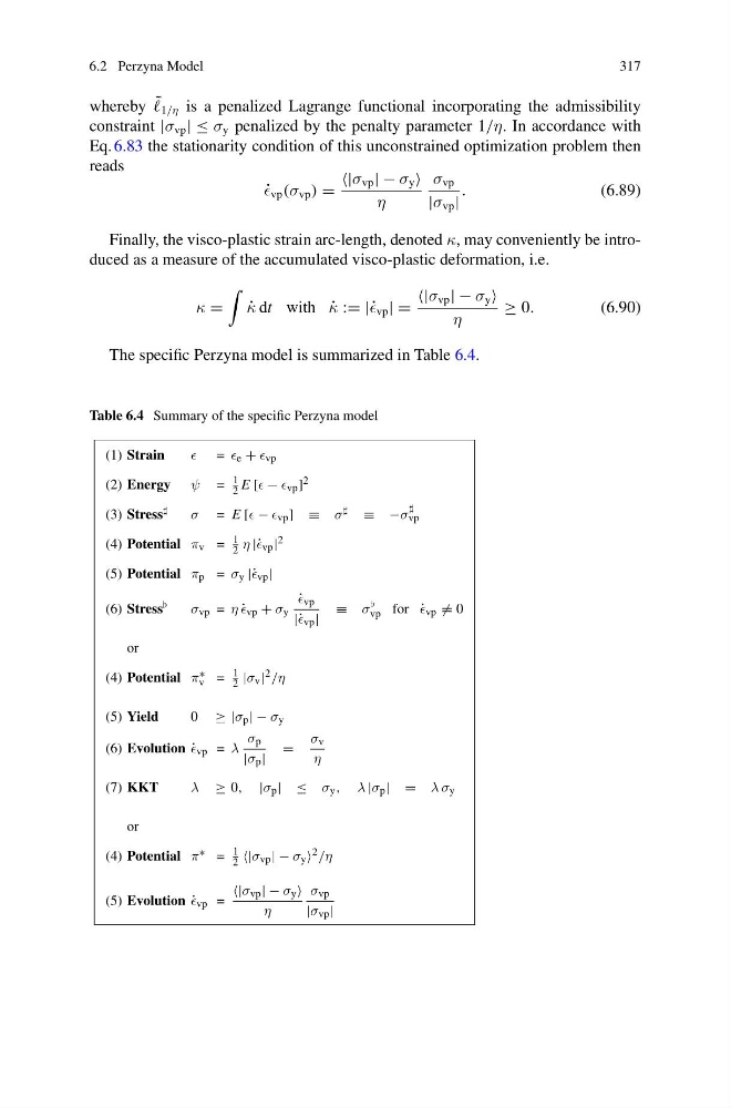
The specific Perzyna model is summarized in Table 6.4.
Table 6.4 Summary of the specific Perzyna model
(1) Strain
= e + vp
(2) Energy ψ =
1
2 E [ − vp ] 2
(3) Stress
σ = E [ − vp ] ≡ σ ≡ −σ
vp
(4) Potential π v =
1
2 η |˙ vp | 2
(5) Potential π p = σ y |˙ vp |
(6) Stress
σ vp = η ˙
vp + σ y
˙
vp
|˙ vp |
≡ σ
vp for ˙
vp = 0
or
(4) Potential π ∗
v =
1
2 |σ v | 2 /η
(5) Yield
0 ≥ |σ p | − σ y
(6) Evolution ˙
vp = λ
σ p
|σ p |
=
σ v
η
(7) KKT
λ ≥ 0, |σ p | ≤ σ y , λ |σ p | = λ σ y
or
(4) Potential π ∗ =
1
2 |σ vp | − σ y 2 /η
(5) Evolution ˙
vp =
|σ vp | − σ y
η
σ vp
|σ vp |
317
whereby ˜
1/η is a penalized Lagrange functional incorporating the admissibility
constraint |σ vp | ≤ σ y penalized by the penalty parameter 1/η. In accordance with
Eq. 6.83 the stationarity condition of this unconstrained optimization problem then
reads
˙
vp (σ vp ) =
|σ vp | − σ y
η
σ vp
|σ vp |
.
(6.89)
Finally, the visco-plastic strain arc-length, denoted κ, may conveniently be introduced as a measure of the accumulated visco-plastic deformation, i.e.
κ =
˙
κ dt with ˙
κ := |˙ vp | =
|σ vp | − σ y
η
≥ 0.
(6.90)
The specific Perzyna model is summarized in Table 6.4.
Table 6.4 Summary of the specific Perzyna model
(1) Strain
= e + vp
(2) Energy ψ =
1
2 E [ − vp ] 2
(3) Stress
σ = E [ − vp ] ≡ σ ≡ −σ
vp
(4) Potential π v =
1
2 η |˙ vp | 2
(5) Potential π p = σ y |˙ vp |
(6) Stress
σ vp = η ˙
vp + σ y
˙
vp
|˙ vp |
≡ σ
vp for ˙
vp = 0
or
(4) Potential π ∗
v =
1
2 |σ v | 2 /η
(5) Yield
0 ≥ |σ p | − σ y
(6) Evolution ˙
vp = λ
σ p
|σ p |
=
σ v
η
(7) KKT
λ ≥ 0, |σ p | ≤ σ y , λ |σ p | = λ σ y
or
(4) Potential π ∗ =
1
2 |σ vp | − σ y 2 /η
(5) Evolution ˙
vp =
|σ vp | − σ y
η
σ vp
|σ vp |