

5.3 Prandtl Hardening Model
267
d(σ p , σ hi , σ hk ; ˙
p , ˙
hi , ˙
hk ) ≥
(5.190)
d(σ
p , σ
hi , σ
hk ; ˙
p , ˙
hi , ˙
hk ) ∀{σ
p , σ
hi , σ
hk } ∈ A,
whereby {σ
p , σ
hi , σ
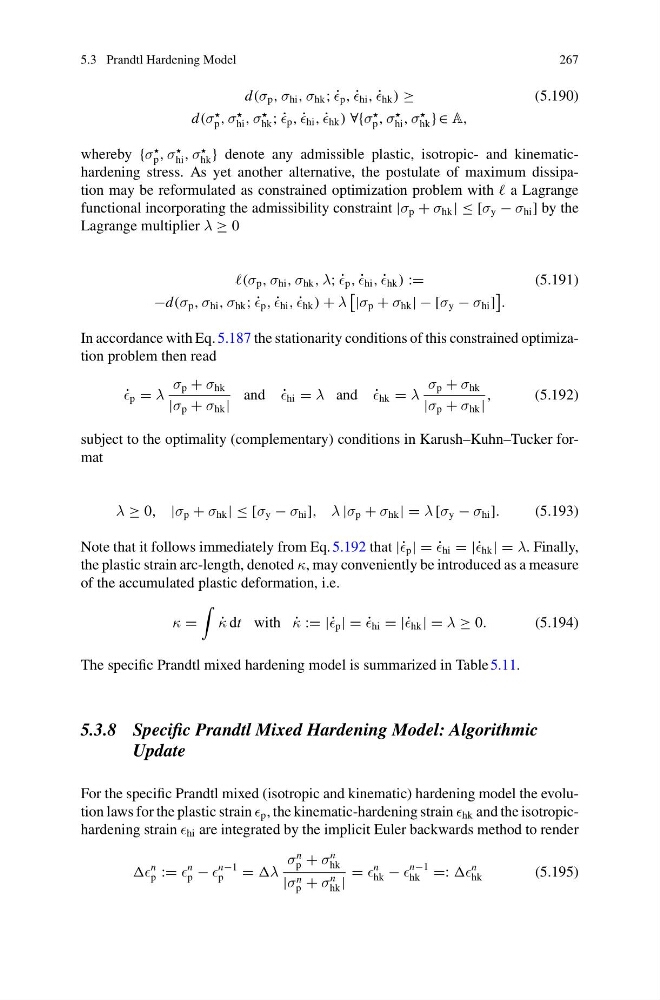
hk } denote any admissible plastic, isotropic- and kinematichardening stress. As yet another alternative, the postulate of maximum dissipation may be reformulated as constrained optimization problem with a Lagrange
functional incorporating the admissibility constraint |σ p + σ hk | ≤ [σ y − σ hi ] by the
Lagrange multiplier λ ≥ 0
(σ p , σ hi , σ hk , λ; ˙
p , ˙
hi , ˙
hk ) :=
(5.191)
−d(σ p , σ hi , σ hk ; ˙
p , ˙
hi , ˙
hk ) + λ
|σ p + σ hk | − [σ y − σ hi ]
.
In accordance with Eq. 5.187 the stationarity conditions of this constrained optimization problem then read
˙
p = λ
σ p + σ hk
|σ p + σ hk |
and ˙
hi = λ and ˙
hk = λ
σ p + σ hk
|σ p + σ hk |
,
(5.192)
subject to the optimality (complementary) conditions in Karush–Kuhn–Tucker format
λ ≥ 0, |σ p + σ hk | ≤ [σ y − σ hi ], λ |σ p + σ hk | = λ [σ y − σ hi ].
(5.193)
Note that it follows immediately from Eq. 5.192 that |˙ p | = ˙
hi = |˙ hk | = λ. Finally,
the plastic strain arc-length, denoted κ, may conveniently be introduced as a measure
of the accumulated plastic deformation, i.e.
κ =
˙
κ dt with ˙
κ := |˙ p | = ˙
hi = |˙ hk | = λ ≥ 0.
(5.194)
The specific Prandtl mixed hardening model is summarized in Table 5.11.
5.3.8 Specific Prandtl Mixed Hardening Model: Algorithmic
Update
For the specific Prandtl mixed (isotropic and kinematic) hardening model the evolution laws for the plastic strain p , the kinematic-hardening strain hk and the isotropichardening strain hi are integrated by the implicit Euler backwards method to render
n
p :=
n
p −
n−1
p
= λ
σ
n
p + σ
n
hk
|σ n
p + σ
n
hk |
=
n
hk −
n−1
hk =:
n
hk
(5.195)
267
d(σ p , σ hi , σ hk ; ˙
p , ˙
hi , ˙
hk ) ≥
(5.190)
d(σ
p , σ
hi , σ
hk ; ˙
p , ˙
hi , ˙
hk ) ∀{σ
p , σ
hi , σ
hk } ∈ A,
whereby {σ
p , σ
hi , σ
hk } denote any admissible plastic, isotropic- and kinematichardening stress. As yet another alternative, the postulate of maximum dissipation may be reformulated as constrained optimization problem with a Lagrange
functional incorporating the admissibility constraint |σ p + σ hk | ≤ [σ y − σ hi ] by the
Lagrange multiplier λ ≥ 0
(σ p , σ hi , σ hk , λ; ˙
p , ˙
hi , ˙
hk ) :=
(5.191)
−d(σ p , σ hi , σ hk ; ˙
p , ˙
hi , ˙
hk ) + λ
|σ p + σ hk | − [σ y − σ hi ]
.
In accordance with Eq. 5.187 the stationarity conditions of this constrained optimization problem then read
˙
p = λ
σ p + σ hk
|σ p + σ hk |
and ˙
hi = λ and ˙
hk = λ
σ p + σ hk
|σ p + σ hk |
,
(5.192)
subject to the optimality (complementary) conditions in Karush–Kuhn–Tucker format
λ ≥ 0, |σ p + σ hk | ≤ [σ y − σ hi ], λ |σ p + σ hk | = λ [σ y − σ hi ].
(5.193)
Note that it follows immediately from Eq. 5.192 that |˙ p | = ˙
hi = |˙ hk | = λ. Finally,
the plastic strain arc-length, denoted κ, may conveniently be introduced as a measure
of the accumulated plastic deformation, i.e.
κ =
˙
κ dt with ˙
κ := |˙ p | = ˙
hi = |˙ hk | = λ ≥ 0.
(5.194)
The specific Prandtl mixed hardening model is summarized in Table 5.11.
5.3.8 Specific Prandtl Mixed Hardening Model: Algorithmic
Update
For the specific Prandtl mixed (isotropic and kinematic) hardening model the evolution laws for the plastic strain p , the kinematic-hardening strain hk and the isotropichardening strain hi are integrated by the implicit Euler backwards method to render
n
p :=
n
p −
n−1
p
= λ
σ
n
p + σ
n
hk
|σ n
p + σ
n
hk |
=
n
hk −
n−1
hk =:
n
hk
(5.195)