

234
5 Plasticity
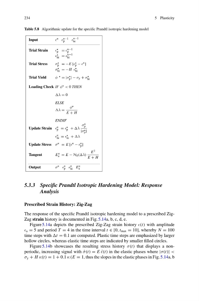
Table 5.8 Algorithmic update for the specific Prandtl isotropic hardening model
Input
n n−1
p
n−1
hi
Trial Strain
p = n−1
p
hi =
n−1
hi
Trial Stress
σ
p = −E [
p − n ]
σ
hi = −H
hi
Trial Yield
φ = |σ
p | − σ y + σ
hi
Loading Check IF φ < 0 THEN
λ = 0
ELSE
λ =
φ
E + H
ENDIF
Update Strain n
p =
p + λ
σ
p
|σ
p |
n
hi =
hi + λ
Update Stress σ n = E [ n − n
p ]
Tangent
E n
a = E − H 0 ((λ)
E 2
E + H
Output
σ n n
p n
hi E n
a
5.3.3 Specific Prandtl Isotropic Hardening Model: Response
Analysis
Prescribed Strain History: Zig-Zag
The response of the specific Prandtl isotropic hardening model to a prescribed ZigZag strain history is documented in Fig. 5.14a, b, c, d, e.
Figure 5.14a depicts the prescribed Zig-Zag strain history (t) with amplitude
a = 5 and period T = 4 in the time interval t ∈ [0, t max = 10], whereby N = 100
time steps with t = 0.1 are computed. Plastic time steps are emphasized by larger
hollow circles, whereas elastic time steps are indicated by smaller filled circles.
Figure 5.14b showcases the resulting stress history σ(t) that displays a nonperiodic, increasing signal with ˙
σ(t) = E ˙
(t) in the elastic phases where |σ(t)| <
σ y + H κ(t) = 1 + 0.1 κ (E = 1, thus the slopes in the elastic phases in Fig. 5.14a, b
5 Plasticity
Table 5.8 Algorithmic update for the specific Prandtl isotropic hardening model
Input
n n−1
p
n−1
hi
Trial Strain
p = n−1
p
hi =
n−1
hi
Trial Stress
σ
p = −E [
p − n ]
σ
hi = −H
hi
Trial Yield
φ = |σ
p | − σ y + σ
hi
Loading Check IF φ < 0 THEN
λ = 0
ELSE
λ =
φ
E + H
ENDIF
Update Strain n
p =
p + λ
σ
p
|σ
p |
n
hi =
hi + λ
Update Stress σ n = E [ n − n
p ]
Tangent
E n
a = E − H 0 ((λ)
E 2
E + H
Output
σ n n
p n
hi E n
a
5.3.3 Specific Prandtl Isotropic Hardening Model: Response
Analysis
Prescribed Strain History: Zig-Zag
The response of the specific Prandtl isotropic hardening model to a prescribed ZigZag strain history is documented in Fig. 5.14a, b, c, d, e.
Figure 5.14a depicts the prescribed Zig-Zag strain history (t) with amplitude
a = 5 and period T = 4 in the time interval t ∈ [0, t max = 10], whereby N = 100
time steps with t = 0.1 are computed. Plastic time steps are emphasized by larger
hollow circles, whereas elastic time steps are indicated by smaller filled circles.
Figure 5.14b showcases the resulting stress history σ(t) that displays a nonperiodic, increasing signal with ˙
σ(t) = E ˙
(t) in the elastic phases where |σ(t)| <
σ y + H κ(t) = 1 + 0.1 κ (E = 1, thus the slopes in the elastic phases in Fig. 5.14a, b