

5.3 Prandtl Hardening Model
233
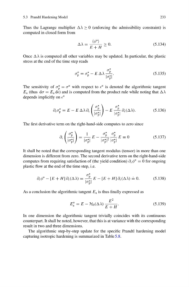
Thus the Lagrange multiplier λ ≥ 0 (enforcing the admissibility constraint) is
computed in closed form from
λ =
φ
E + H
≥ 0.
(5.134)
Once λ is computed all other variables may be updated. In particular, the plastic
stress at the end of the time step reads
σ
n
p = σ
p − E λ
σ
p
|σ
p |
.
(5.135)
The sensitivity of σ
n
p = σ
n with respect to
n is denoted the algorithmic tangent
E a (thus dσ = E a d) and is computed from the product rule while noting that λ
depends implicitly on
n
∂ σ
n
p = E − E λ ∂
σ
p
|σ
p |
− E
σ
p
|σ
p |
∂ ((λ).
(5.136)
The first derivative term on the right-hand-side computes to zero since
∂
σ
p
|σ
p |
=
1
|σ
p |
E −
σ
p
|σ
p | 2
σ
p
|σ
p |
E ≡ 0
(5.137)
It shall be noted that the corresponding tangent modulus (tensor) in more than one
dimension is different from zero. The second derivative term on the right-hand-side
computes from requiring satisfaction of (the yield condition) ∂ φ
n
= 0 for ongoing
plastic flow at the end of the time step, i.e.
∂ φ
− [E + H ] ∂ ((λ) =
σ
p
|σ
p |
E − [E + H ] ∂ ((λ)
.
= 0.
(5.138)
As a conclusion the algorithmic tangent E a is thus finally expressed as
E
n
a = E − H 0 ((λ)
E
2
E + H
.
(5.139)
In one dimension the algorithmic tangent trivially coincides with its continuous
counterpart. It shall be noted, however, that this is at variance with the corresponding
result in two and three dimensions.
The algorithmic step-by-step update for the specific Prandtl hardening model
capturing isotropic hardening is summarized in Table 5.8.
233
Thus the Lagrange multiplier λ ≥ 0 (enforcing the admissibility constraint) is
computed in closed form from
λ =
φ
E + H
≥ 0.
(5.134)
Once λ is computed all other variables may be updated. In particular, the plastic
stress at the end of the time step reads
σ
n
p = σ
p − E λ
σ
p
|σ
p |
.
(5.135)
The sensitivity of σ
n
p = σ
n with respect to
n is denoted the algorithmic tangent
E a (thus dσ = E a d) and is computed from the product rule while noting that λ
depends implicitly on
n
∂ σ
n
p = E − E λ ∂
σ
p
|σ
p |
− E
σ
p
|σ
p |
∂ ((λ).
(5.136)
The first derivative term on the right-hand-side computes to zero since
∂
σ
p
|σ
p |
=
1
|σ
p |
E −
σ
p
|σ
p | 2
σ
p
|σ
p |
E ≡ 0
(5.137)
It shall be noted that the corresponding tangent modulus (tensor) in more than one
dimension is different from zero. The second derivative term on the right-hand-side
computes from requiring satisfaction of (the yield condition) ∂ φ
n
= 0 for ongoing
plastic flow at the end of the time step, i.e.
∂ φ
− [E + H ] ∂ ((λ) =
σ
p
|σ
p |
E − [E + H ] ∂ ((λ)
.
= 0.
(5.138)
As a conclusion the algorithmic tangent E a is thus finally expressed as
E
n
a = E − H 0 ((λ)
E
2
E + H
.
(5.139)
In one dimension the algorithmic tangent trivially coincides with its continuous
counterpart. It shall be noted, however, that this is at variance with the corresponding
result in two and three dimensions.
The algorithmic step-by-step update for the specific Prandtl hardening model
capturing isotropic hardening is summarized in Table 5.8.