

10
1 Introduction
σ
σ
σ
σ
σ
σ
1
2
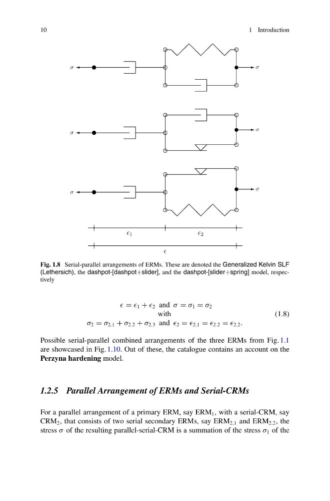
Fig. 1.8 Serial-parallel arrangements of ERMs. These are denoted the Generalized Kelvin SLF
(Lethersich), the dashpot-[dashpot+slider], and the dashpot-[slider+spring] model, respectively
= 1 + 2 and σ = σ 1 = σ 2
with
σ 2 = σ 2.1 + σ 2.2 + σ 2.3 and 2 = 2.1 = 2.2 = 2.2 .
(1.8)
Possible serial-parallel combined arrangements of the three ERMs from Fig. 1.1
are showcased in Fig. 1.10. Out of these, the catalogue contains an account on the
Perzyna hardening model.
1.2.5 Parallel Arrangement of ERMs and Serial-CRMs
For a parallel arrangement of a primary ERM, say ERM 1 , with a serial-CRM, say
CRM 2 , that consists of two serial secondary ERMs, say ERM 2.1 and ERM 2.2 , the
stress σ of the resulting parallel-serial-CRM is a summation of the stress σ 1 of the
1 Introduction
σ
σ
σ
σ
σ
σ
1
2
Fig. 1.8 Serial-parallel arrangements of ERMs. These are denoted the Generalized Kelvin SLF
(Lethersich), the dashpot-[dashpot+slider], and the dashpot-[slider+spring] model, respectively
= 1 + 2 and σ = σ 1 = σ 2
with
σ 2 = σ 2.1 + σ 2.2 + σ 2.3 and 2 = 2.1 = 2.2 = 2.2 .
(1.8)
Possible serial-parallel combined arrangements of the three ERMs from Fig. 1.1
are showcased in Fig. 1.10. Out of these, the catalogue contains an account on the
Perzyna hardening model.
1.2.5 Parallel Arrangement of ERMs and Serial-CRMs
For a parallel arrangement of a primary ERM, say ERM 1 , with a serial-CRM, say
CRM 2 , that consists of two serial secondary ERMs, say ERM 2.1 and ERM 2.2 , the
stress σ of the resulting parallel-serial-CRM is a summation of the stress σ 1 of the