

178
4 Visco-Elasticity
σ
σ
˜ e
˜ v
E 0 := E m + E ∞
η k := η m [E m + E ∞ ]
2
/E
2
m
E k := E ∞ [E m + E ∞ ]/E m
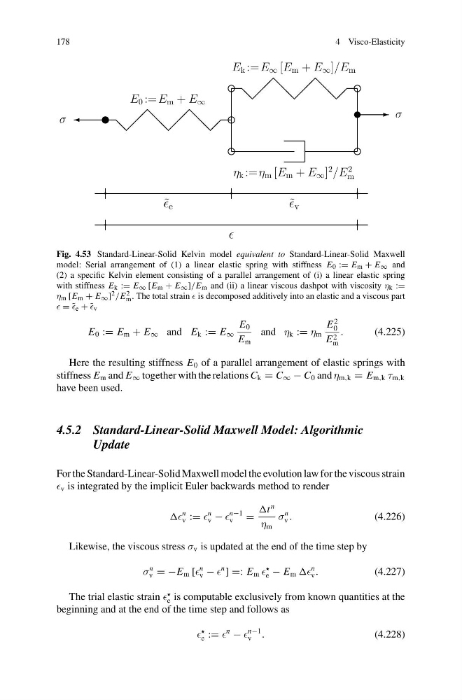
Fig. 4.53 Standard-Linear-Solid Kelvin model equivalent to Standard-Linear-Solid Maxwell
model: Serial arrangement of (1) a linear elastic spring with stiffness E 0 := E m + E ∞ and
(2) a specific Kelvin element consisting of a parallel arrangement of (i) a linear elastic spring
with stiffness E k := E ∞ [E m + E ∞ ]/E m and (ii) a linear viscous dashpot with viscosity η k :=
η m [E m + E ∞ ] 2 /E 2
m . The total strain is decomposed additively into an elastic and a viscous part
= ˜
e + ˜
v
E 0 := E m + E ∞ and E k := E ∞
E 0
E m
and η k := η m
E
2
0
E 2
m
.
(4.225)
Here the resulting stiffness E 0 of a parallel arrangement of elastic springs with
stiffness E m and E ∞ together with the relations C k = C ∞ − C 0 and η m,k = E m,k τ m,k
have been used.
4.5.2 Standard-Linear-Solid Maxwell Model: Algorithmic
Update
For the Standard-Linear-Solid Maxwell model the evolution law for the viscous strain
v is integrated by the implicit Euler backwards method to render
n
v :=
n
v −
n−1
v
=
n
η m
σ
n
v .
(4.226)
Likewise, the viscous stress σ v is updated at the end of the time step by
σ
n
v = −E m [
n
v −
n
] =: E m
e − E m
n
v .
(4.227)
The trial elastic strain
e is computable exclusively from known quantities at the
beginning and at the end of the time step and follows as
e :=
n
−
n−1
v .
(4.228)
4 Visco-Elasticity
σ
σ
˜ e
˜ v
E 0 := E m + E ∞
η k := η m [E m + E ∞ ]
2
/E
2
m
E k := E ∞ [E m + E ∞ ]/E m
Fig. 4.53 Standard-Linear-Solid Kelvin model equivalent to Standard-Linear-Solid Maxwell
model: Serial arrangement of (1) a linear elastic spring with stiffness E 0 := E m + E ∞ and
(2) a specific Kelvin element consisting of a parallel arrangement of (i) a linear elastic spring
with stiffness E k := E ∞ [E m + E ∞ ]/E m and (ii) a linear viscous dashpot with viscosity η k :=
η m [E m + E ∞ ] 2 /E 2
m . The total strain is decomposed additively into an elastic and a viscous part
= ˜
e + ˜
v
E 0 := E m + E ∞ and E k := E ∞
E 0
E m
and η k := η m
E
2
0
E 2
m
.
(4.225)
Here the resulting stiffness E 0 of a parallel arrangement of elastic springs with
stiffness E m and E ∞ together with the relations C k = C ∞ − C 0 and η m,k = E m,k τ m,k
have been used.
4.5.2 Standard-Linear-Solid Maxwell Model: Algorithmic
Update
For the Standard-Linear-Solid Maxwell model the evolution law for the viscous strain
v is integrated by the implicit Euler backwards method to render
n
v :=
n
v −
n−1
v
=
n
η m
σ
n
v .
(4.226)
Likewise, the viscous stress σ v is updated at the end of the time step by
σ
n
v = −E m [
n
v −
n
] =: E m
e − E m
n
v .
(4.227)
The trial elastic strain
e is computable exclusively from known quantities at the
beginning and at the end of the time step and follows as
e :=
n
−
n−1
v .
(4.228)