

154
4 Visco-Elasticity
4.4.2 Specific Maxwell Model: Algorithmic Update
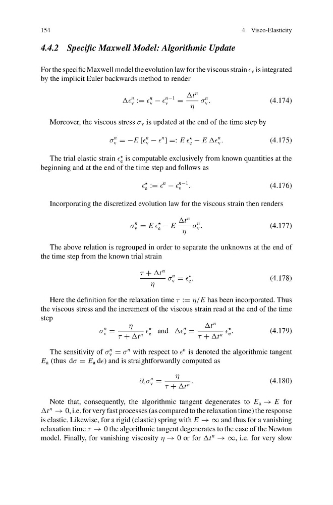
For the specific Maxwell model the evolution law for the viscous strain v is integrated
by the implicit Euler backwards method to render
n
v :=
n
v −
n−1
v
=
t
n
η
σ
n
v .
(4.174)
Moreover, the viscous stress σ v is updated at the end of the time step by
σ
n
v = −E [
n
v −
n
] =: E
e − E
n
v .
(4.175)
The trial elastic strain
e is computable exclusively from known quantities at the
beginning and at the end of the time step and follows as
e :=
n
−
n−1
v .
(4.176)
Incorporating the discretized evolution law for the viscous strain then renders
σ
n
v = E
e − E
t
n
η
σ
n
v .
(4.177)
The above relation is regrouped in order to separate the unknowns at the end of
the time step from the known trial strain
τ + t
n
η
σ
n
v =
e .
(4.178)
Here the definition for the relaxation time τ := η/E has been incorporated. Thus
the viscous stress and the increment of the viscous strain read at the end of the time
step
σ
n
v =
η
τ + t n
e and
n
v =
t
n
τ + t n
e .
(4.179)
The sensitivity of σ
n
v = σ
n with respect to
n is denoted the algorithmic tangent
E a (thus dσ = E a d) and is straightforwardly computed as
∂ σ
n
v =
η
τ + t n .
(4.180)
Note that, consequently, the algorithmic tangent degenerates to E a → E for
t
n
→ 0, i.e. for very fast processes (as compared to the relaxation time) the response
is elastic. Likewise, for a rigid (elastic) spring with E → ∞ and thus for a vanishing
relaxation time τ → 0 the algorithmic tangent degenerates to the case of the Newton
model. Finally, for vanishing viscosity η → 0 or for t
n
→ ∞, i.e. for very slow
4 Visco-Elasticity
4.4.2 Specific Maxwell Model: Algorithmic Update
For the specific Maxwell model the evolution law for the viscous strain v is integrated
by the implicit Euler backwards method to render
n
v :=
n
v −
n−1
v
=
t
n
η
σ
n
v .
(4.174)
Moreover, the viscous stress σ v is updated at the end of the time step by
σ
n
v = −E [
n
v −
n
] =: E
e − E
n
v .
(4.175)
The trial elastic strain
e is computable exclusively from known quantities at the
beginning and at the end of the time step and follows as
e :=
n
−
n−1
v .
(4.176)
Incorporating the discretized evolution law for the viscous strain then renders
σ
n
v = E
e − E
t
n
η
σ
n
v .
(4.177)
The above relation is regrouped in order to separate the unknowns at the end of
the time step from the known trial strain
τ + t
n
η
σ
n
v =
e .
(4.178)
Here the definition for the relaxation time τ := η/E has been incorporated. Thus
the viscous stress and the increment of the viscous strain read at the end of the time
step
σ
n
v =
η
τ + t n
e and
n
v =
t
n
τ + t n
e .
(4.179)
The sensitivity of σ
n
v = σ
n with respect to
n is denoted the algorithmic tangent
E a (thus dσ = E a d) and is straightforwardly computed as
∂ σ
n
v =
η
τ + t n .
(4.180)
Note that, consequently, the algorithmic tangent degenerates to E a → E for
t
n
→ 0, i.e. for very fast processes (as compared to the relaxation time) the response
is elastic. Likewise, for a rigid (elastic) spring with E → ∞ and thus for a vanishing
relaxation time τ → 0 the algorithmic tangent degenerates to the case of the Newton
model. Finally, for vanishing viscosity η → 0 or for t
n
→ ∞, i.e. for very slow