

4.4 Maxwell Model
153
10
−3 10
−2 10
−1 10
0 10
1 10
2 10
3
10
−5
10
−4
10
−3
10
−2
10
−1
10
0
ω
E a
E
τ = 10
2
, 10
1
, 10
0
, 10
−1
, 10
−2
ωτ
√
1 + ω 2 τ 2
10
−3 10
−2 10
−1 10
0 10
1 10
2 10
3
10
−6
10
−3
10
0
10
3
10
6
ω
E
E
τ = 10
2
, 10
1
, 10
0
, 10
−1
, 10
−2
1
ωτ
10
−3 10
−2 10
−1 10
0 10
1 10
2 10
3
10
0
10
1
10
2
10
3
10
4
10
5
ω
C a
C
τ = 10
2
, 10
1
, 10
0
, 10
−1
, 10
−2
√
1 + ω 2 τ 2
ωτ
10
−3 10
−2 10
−1 10
0 10
1 10
2 10
3
10
−6
10
−3
10
0
10
3
10
6
ω
C
C
τ = 10
2
, 10
1
, 10
0
, 10
−1
, 10
−2
1
ωτ
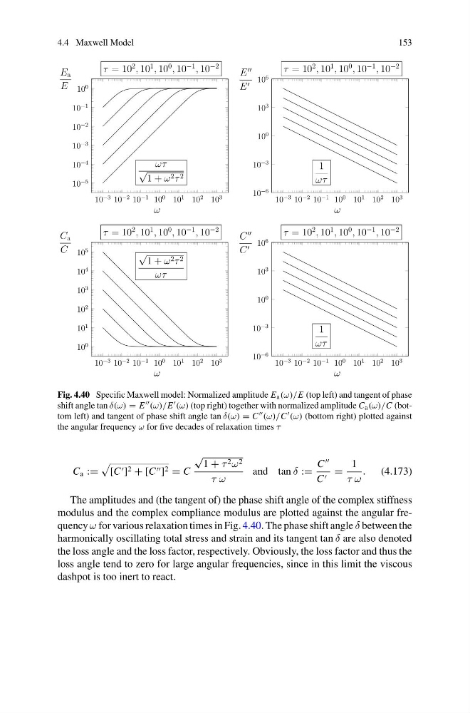
Fig. 4.40 Specific Maxwell model: Normalized amplitude E a (ω)/E (top left) and tangent of phase
shift angle tan δ(ω) = E (ω)/E (ω) (top right) together with normalized amplitude C a (ω)/C (bottom left) and tangent of phase shift angle tan δ(ω) = C (ω)/C (ω) (bottom right) plotted against
the angular frequency ω for five decades of relaxation times τ
C a :=
[C ] 2 + [C ] 2 = C
√
1 + τ 2 ω 2
τ ω
and tan δ :=
C
C =
1
τ ω
. (4.173)
The amplitudes and (the tangent of) the phase shift angle of the complex stiffness
modulus and the complex compliance modulus are plotted against the angular frequency ω for various relaxation times in Fig. 4.40. The phase shift angle δ between the
harmonically oscillating total stress and strain and its tangent tan δ are also denoted
the loss angle and the loss factor, respectively. Obviously, the loss factor and thus the
loss angle tend to zero for large angular frequencies, since in this limit the viscous
dashpot is too inert to react.
153
10
−3 10
−2 10
−1 10
0 10
1 10
2 10
3
10
−5
10
−4
10
−3
10
−2
10
−1
10
0
ω
E a
E
τ = 10
2
, 10
1
, 10
0
, 10
−1
, 10
−2
ωτ
√
1 + ω 2 τ 2
10
−3 10
−2 10
−1 10
0 10
1 10
2 10
3
10
−6
10
−3
10
0
10
3
10
6
ω
E
E
τ = 10
2
, 10
1
, 10
0
, 10
−1
, 10
−2
1
ωτ
10
−3 10
−2 10
−1 10
0 10
1 10
2 10
3
10
0
10
1
10
2
10
3
10
4
10
5
ω
C a
C
τ = 10
2
, 10
1
, 10
0
, 10
−1
, 10
−2
√
1 + ω 2 τ 2
ωτ
10
−3 10
−2 10
−1 10
0 10
1 10
2 10
3
10
−6
10
−3
10
0
10
3
10
6
ω
C
C
τ = 10
2
, 10
1
, 10
0
, 10
−1
, 10
−2
1
ωτ
Fig. 4.40 Specific Maxwell model: Normalized amplitude E a (ω)/E (top left) and tangent of phase
shift angle tan δ(ω) = E (ω)/E (ω) (top right) together with normalized amplitude C a (ω)/C (bottom left) and tangent of phase shift angle tan δ(ω) = C (ω)/C (ω) (bottom right) plotted against
the angular frequency ω for five decades of relaxation times τ
C a :=
[C ] 2 + [C ] 2 = C
√
1 + τ 2 ω 2
τ ω
and tan δ :=
C
C =
1
τ ω
. (4.173)
The amplitudes and (the tangent of) the phase shift angle of the complex stiffness
modulus and the complex compliance modulus are plotted against the angular frequency ω for various relaxation times in Fig. 4.40. The phase shift angle δ between the
harmonically oscillating total stress and strain and its tangent tan δ are also denoted
the loss angle and the loss factor, respectively. Obviously, the loss factor and thus the
loss angle tend to zero for large angular frequencies, since in this limit the viscous
dashpot is too inert to react.