

4.4 Maxwell Model
145
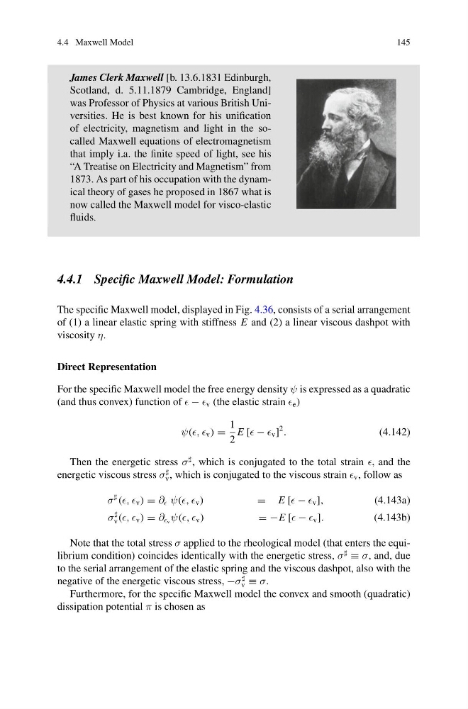
James Clerk Maxwell [b. 13.6.1831 Edinburgh,
Scotland, d. 5.11.1879 Cambridge, England]
was Professor of Physics at various British Universities. He is best known for his unification
of electricity, magnetism and light in the socalled Maxwell equations of electromagnetism
that imply i.a. the finite speed of light, see his
“A Treatise on Electricity and Magnetism” from
1873. As part of his occupation with the dynamical theory of gases he proposed in 1867 what is
now called the Maxwell model for visco-elastic
fluids.
4.4.1 Specific Maxwell Model: Formulation
The specific Maxwell model, displayed in Fig. 4.36, consists of a serial arrangement
of (1) a linear elastic spring with stiffness E and (2) a linear viscous dashpot with
viscosity η.
Direct Representation
For the specific Maxwell model the free energy density ψ is expressed as a quadratic
(and thus convex) function of − v (the elastic strain e )
ψ(, v ) =
1
2
E [ − v ]
2
.
(4.142)
Then the energetic stress σ
, which is conjugated to the total strain , and the
energetic viscous stress σ
v , which is conjugated to the viscous strain v , follow as
σ
(, v ) = ∂ ψ(, v )
= E [ − v ],
(4.143a)
σ
v (, v ) = ∂ v ψ(, v )
= −E [ − v ].
(4.143b)
Note that the total stress σ applied to the rheological model (that enters the equilibrium condition) coincides identically with the energetic stress, σ
≡ σ, and, due
to the serial arrangement of the elastic spring and the viscous dashpot, also with the
negative of the energetic viscous stress, −σ
v ≡ σ.
Furthermore, for the specific Maxwell model the convex and smooth (quadratic)
dissipation potential π is chosen as
145
James Clerk Maxwell [b. 13.6.1831 Edinburgh,
Scotland, d. 5.11.1879 Cambridge, England]
was Professor of Physics at various British Universities. He is best known for his unification
of electricity, magnetism and light in the socalled Maxwell equations of electromagnetism
that imply i.a. the finite speed of light, see his
“A Treatise on Electricity and Magnetism” from
1873. As part of his occupation with the dynamical theory of gases he proposed in 1867 what is
now called the Maxwell model for visco-elastic
fluids.
4.4.1 Specific Maxwell Model: Formulation
The specific Maxwell model, displayed in Fig. 4.36, consists of a serial arrangement
of (1) a linear elastic spring with stiffness E and (2) a linear viscous dashpot with
viscosity η.
Direct Representation
For the specific Maxwell model the free energy density ψ is expressed as a quadratic
(and thus convex) function of − v (the elastic strain e )
ψ(, v ) =
1
2
E [ − v ]
2
.
(4.142)
Then the energetic stress σ
, which is conjugated to the total strain , and the
energetic viscous stress σ
v , which is conjugated to the viscous strain v , follow as
σ
(, v ) = ∂ ψ(, v )
= E [ − v ],
(4.143a)
σ
v (, v ) = ∂ v ψ(, v )
= −E [ − v ].
(4.143b)
Note that the total stress σ applied to the rheological model (that enters the equilibrium condition) coincides identically with the energetic stress, σ
≡ σ, and, due
to the serial arrangement of the elastic spring and the viscous dashpot, also with the
negative of the energetic viscous stress, −σ
v ≡ σ.
Furthermore, for the specific Maxwell model the convex and smooth (quadratic)
dissipation potential π is chosen as