

4.3 Generalized-Kelvin Model
143
σ
(•) = ∂ ˙
π (•) and σ
v k
(•) = ∂ ˙
v k
π (•) (• = ˙
, { ˙
v j } \1 ).
(4.136b)
Alternatively, after re-parametrization (˙ v 1 = ˙
− ˙
v and σ v k = σ
+ σ
v k
), the stationarity conditions corresponding to Eqs. 4.135a and 4.135b read more conventiently
˙
v 1 (σ v 1 ) = ∂ σ v 1 ¯
π
∗
1 (σ v 1 ) and ˙
v k (σ v k ) = ∂ σ v k ¯
π
∗
k (σ v k ),
(4.137a)
σ v 1 ( ˙
v 1 ) = ∂ ˙
v 1
¯
π 1 ( ˙
v 1 ) and σ v k ( ˙
v k ) = ∂ ˙
v k
¯
π k ( ˙
v k ).
(4.137b)
Obviously, the relations in Eqs. 4.136a and 4.136b (or likewise in Eqs. 4.137a and
4.137b) determine entirely the dissipative behavior of the generic Generalized-Kelvin
model, thus the formulation is completed at this stage.
Finally, as a further interesting aspect, the dissipation for the generic GeneralizedKelvin model follows as the sum
d(σ
, {σ
v j
} \1 , ˙
{ ˙
v j } \1 ) = d 1 (σ
, ˙
+
K
k=2
d k (σ
v k
, ˙
v k ) ≥ 0.
(4.138)
Alternatively, after re-parametrization (˙ v 1 = ˙
− ˙
v and σ v k = σ
+ σ
v k
), the dissipation reads
d(σ
, {σ
v j
} \1 , ˙
{ ˙
v j } \1 ) = ¯
d 1 (σ v 1 , ˙
v 1 ) +
K
k=2
¯
d k (σ v k , ˙
v k ) ≥ 0.
(4.139)
Thereby, the re-parameterized dissipation ¯
d 1 = σ v 1 ˙
v 1 and ¯
d k = σ v k ˙
v k (k =
2, . . . , K ) for each generic Kelvin element is alternatively expressed from Eqs. 4.135a
and 4.135b in terms of the dissipation potentials ¯
π 1 , ¯
π k and the dual dissipation potentials ¯
π
∗
1 , ¯
π
∗
k as
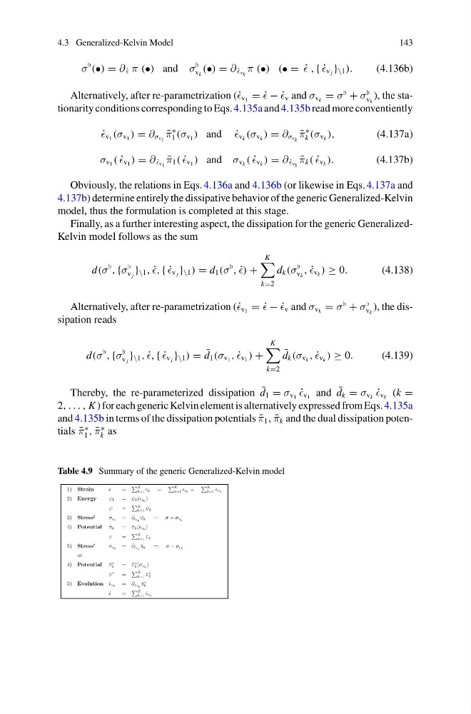
Table 4.9 Summary of the generic Generalized-Kelvin model
1) Strain
=
K
k=1 k
=
K
k=1 ek =
K
k=1 vk
2) Energy
ψk = ψk( ek )
ψ
=
K
k=1 ψk
3) Stress
σe k = ∂ ek ψk =: σ − σv k
4) Potential ¯
πk = ¯
πk(˙v k )
π
=
K
k=1 ¯
πk
5) Stress
σv k = ∂˙ vk ¯
πk =: σ − σe k
or
4) Potential ¯
π
∗
k
= ¯
π
∗
k (σv k )
π
∗
=
K
k=1 ¯
π
∗
k
5) Evolution ˙v k = ∂σ vk ¯
π
∗
k
˙
=
K
k=1 ˙v k
143
σ
(•) = ∂ ˙
π (•) and σ
v k
(•) = ∂ ˙
v k
π (•) (• = ˙
, { ˙
v j } \1 ).
(4.136b)
Alternatively, after re-parametrization (˙ v 1 = ˙
− ˙
v and σ v k = σ
+ σ
v k
), the stationarity conditions corresponding to Eqs. 4.135a and 4.135b read more conventiently
˙
v 1 (σ v 1 ) = ∂ σ v 1 ¯
π
∗
1 (σ v 1 ) and ˙
v k (σ v k ) = ∂ σ v k ¯
π
∗
k (σ v k ),
(4.137a)
σ v 1 ( ˙
v 1 ) = ∂ ˙
v 1
¯
π 1 ( ˙
v 1 ) and σ v k ( ˙
v k ) = ∂ ˙
v k
¯
π k ( ˙
v k ).
(4.137b)
Obviously, the relations in Eqs. 4.136a and 4.136b (or likewise in Eqs. 4.137a and
4.137b) determine entirely the dissipative behavior of the generic Generalized-Kelvin
model, thus the formulation is completed at this stage.
Finally, as a further interesting aspect, the dissipation for the generic GeneralizedKelvin model follows as the sum
d(σ
, {σ
v j
} \1 , ˙
{ ˙
v j } \1 ) = d 1 (σ
, ˙
+
K
k=2
d k (σ
v k
, ˙
v k ) ≥ 0.
(4.138)
Alternatively, after re-parametrization (˙ v 1 = ˙
− ˙
v and σ v k = σ
+ σ
v k
), the dissipation reads
d(σ
, {σ
v j
} \1 , ˙
{ ˙
v j } \1 ) = ¯
d 1 (σ v 1 , ˙
v 1 ) +
K
k=2
¯
d k (σ v k , ˙
v k ) ≥ 0.
(4.139)
Thereby, the re-parameterized dissipation ¯
d 1 = σ v 1 ˙
v 1 and ¯
d k = σ v k ˙
v k (k =
2, . . . , K ) for each generic Kelvin element is alternatively expressed from Eqs. 4.135a
and 4.135b in terms of the dissipation potentials ¯
π 1 , ¯
π k and the dual dissipation potentials ¯
π
∗
1 , ¯
π
∗
k as
Table 4.9 Summary of the generic Generalized-Kelvin model
1) Strain
=
K
k=1 k
=
K
k=1 ek =
K
k=1 vk
2) Energy
ψk = ψk( ek )
ψ
=
K
k=1 ψk
3) Stress
σe k = ∂ ek ψk =: σ − σv k
4) Potential ¯
πk = ¯
πk(˙v k )
π
=
K
k=1 ¯
πk
5) Stress
σv k = ∂˙ vk ¯
πk =: σ − σe k
or
4) Potential ¯
π
∗
k
= ¯
π
∗
k (σv k )
π
∗
=
K
k=1 ¯
π
∗
k
5) Evolution ˙v k = ∂σ vk ¯
π
∗
k
˙
=
K
k=1 ˙v k