

4.3 Generalized-Kelvin Model
127
10
−3 10
−2 10
−1 10
0 10
1 10
2 10
3
10
0
10
0.1
10
0.2
10
0.3
ω
E
E ∞
τ = 10
2
, 10
1
, 10
0
, 10
−1
, 10
−2
1 + c ω
2
τ
2
1 + c 2 ω 2 τ 2
10
−3 10
−2 10
−1 10
0 10
1 10
2 10
3
10
−5
10
−4
10
−3
10
−2
10
−1
10
0
ω
E
E ∞
τ = 10
2
, 10
1
, 10
0
, 10
−1
, 10
−2
[1 − c] ωτ
1 + c 2 ω 2 τ 2
10
−3 10
−2 10
−1 10
0 10
1 10
2 10
3
10
−0.3
10
−0.2
10
−0.1
10
0
ω
C
C ∞
τ = 10
2
, 10
1
, 10
0
, 10
−1
, 10
−2
1 + c ω
2
τ
2
1 + ω 2 τ 2
10
−3 10
−2 10
−1 10
0 10
1 10
2 10
3
10
−5
10
−4
10
−3
10
−2
10
−1
ω
C
C ∞
τ = 10
2
, 10
1
, 10
0
, 10
−1
, 10
−2
[1 − c] ωτ
1 + ω 2 τ 2
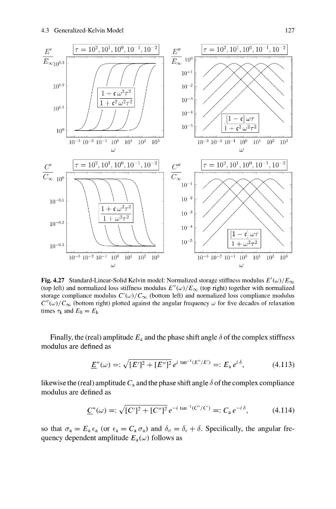
Fig. 4.27 Standard-Linear-Solid Kelvin model: Normalized storage stiffness modulus E (ω)/E ∞
(top left) and normalized loss stiffness modulus E (ω)/E ∞ (top right) together with normalized
storage compliance modulus C (ω)/C ∞ (bottom left) and normalized loss compliance modulus
C (ω)/C ∞ (bottom right) plotted against the angular frequency ω for five decades of relaxation
times τ k and E 0 = E k
Finally, the (real) amplitude E a and the phase shift angle δ of the complex stiffness
modulus are defined as
E
∗
(ω) =:
[E ] 2 + [E ] 2 e
i tan
−1 (E
/E
)
=: E a e
i δ
,
(4.113)
likewise the (real) amplitude C a and the phase shift angle δ of the complex compliance
modulus are defined as
C
∗
(ω) =:
[C ] 2 + [C ] 2 e
−i tan
−1 (C
/C
)
=: C a e
−i δ
,
(4.114)
so that σ a = E a a (or a = C a σ a ) and δ σ = δ + δ. Specifically, the angular frequency dependent amplitude E a (ω) follows as
127
10
−3 10
−2 10
−1 10
0 10
1 10
2 10
3
10
0
10
0.1
10
0.2
10
0.3
ω
E
E ∞
τ = 10
2
, 10
1
, 10
0
, 10
−1
, 10
−2
1 + c ω
2
τ
2
1 + c 2 ω 2 τ 2
10
−3 10
−2 10
−1 10
0 10
1 10
2 10
3
10
−5
10
−4
10
−3
10
−2
10
−1
10
0
ω
E
E ∞
τ = 10
2
, 10
1
, 10
0
, 10
−1
, 10
−2
[1 − c] ωτ
1 + c 2 ω 2 τ 2
10
−3 10
−2 10
−1 10
0 10
1 10
2 10
3
10
−0.3
10
−0.2
10
−0.1
10
0
ω
C
C ∞
τ = 10
2
, 10
1
, 10
0
, 10
−1
, 10
−2
1 + c ω
2
τ
2
1 + ω 2 τ 2
10
−3 10
−2 10
−1 10
0 10
1 10
2 10
3
10
−5
10
−4
10
−3
10
−2
10
−1
ω
C
C ∞
τ = 10
2
, 10
1
, 10
0
, 10
−1
, 10
−2
[1 − c] ωτ
1 + ω 2 τ 2
Fig. 4.27 Standard-Linear-Solid Kelvin model: Normalized storage stiffness modulus E (ω)/E ∞
(top left) and normalized loss stiffness modulus E (ω)/E ∞ (top right) together with normalized
storage compliance modulus C (ω)/C ∞ (bottom left) and normalized loss compliance modulus
C (ω)/C ∞ (bottom right) plotted against the angular frequency ω for five decades of relaxation
times τ k and E 0 = E k
Finally, the (real) amplitude E a and the phase shift angle δ of the complex stiffness
modulus are defined as
E
∗
(ω) =:
[E ] 2 + [E ] 2 e
i tan
−1 (E
/E
)
=: E a e
i δ
,
(4.113)
likewise the (real) amplitude C a and the phase shift angle δ of the complex compliance
modulus are defined as
C
∗
(ω) =:
[C ] 2 + [C ] 2 e
−i tan
−1 (C
/C
)
=: C a e
−i δ
,
(4.114)
so that σ a = E a a (or a = C a σ a ) and δ σ = δ + δ. Specifically, the angular frequency dependent amplitude E a (ω) follows as