

126
4 Visco-Elasticity
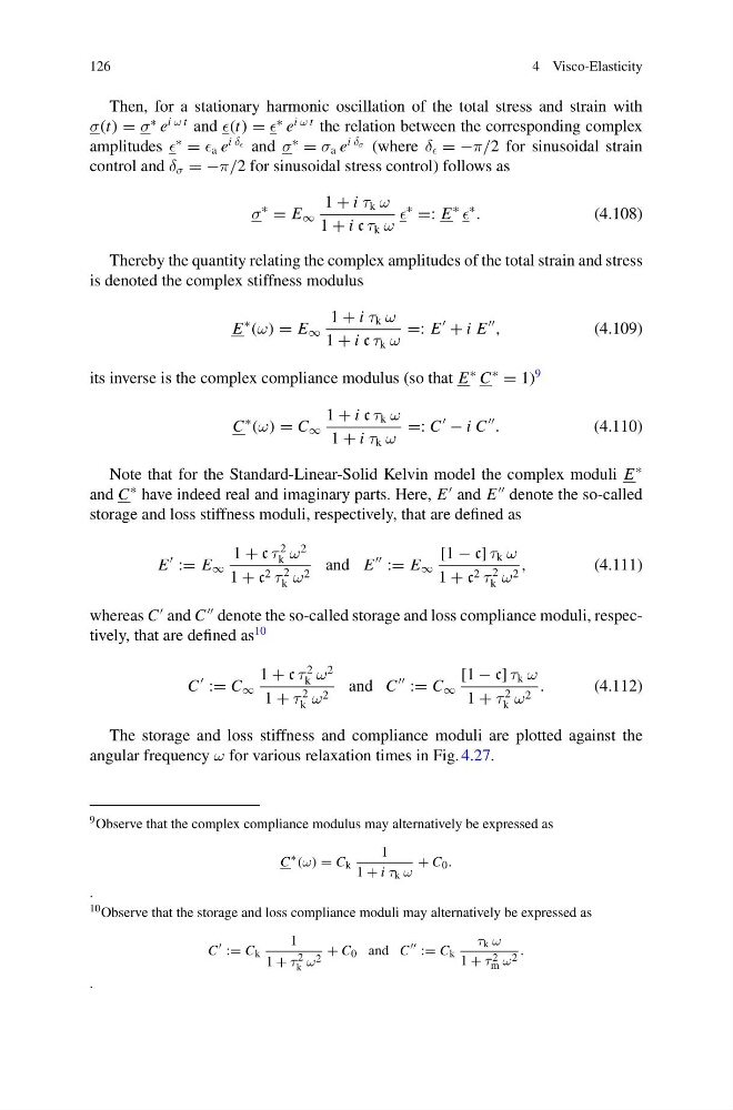
Then, for a stationary harmonic oscillation of the total stress and strain with
σ(t) = σ
∗ e
i ω t and (t) =
∗ e
i ω t the relation between the corresponding complex
amplitudes
∗
= a e
i δ and σ
∗
= σ a e
i δ σ (where δ = −π/2 for sinusoidal strain
control and δ σ = −π/2 for sinusoidal stress control) follows as
σ
∗
= E ∞
1 + i τ k ω
1 + i c τ k ω
∗
=: E
∗
∗
.
(4.108)
Thereby the quantity relating the complex amplitudes of the total strain and stress
is denoted the complex stiffness modulus
E
∗
(ω) = E ∞
1 + i τ k ω
1 + i c τ k ω
=: E
+ i E
,
(4.109)
its inverse is the complex compliance modulus (so that E
∗ C
∗
= 1)
9
C
∗
(ω) = C ∞
1 + i c τ k ω
1 + i τ k ω
=: C
− i C
.
(4.110)
Note that for the Standard-Linear-Solid Kelvin model the complex moduli E
∗
and C
∗ have indeed real and imaginary parts. Here, E
and E
denote the so-called
storage and loss stiffness moduli, respectively, that are defined as
E
:= E ∞
1 + c τ
2
k ω
2
1 + c 2 τ
2
k ω 2 and E
:= E ∞
[1 − c] τ k ω
1 + c 2 τ
2
k ω 2 ,
(4.111)
whereas C
and C
denote the so-called storage and loss compliance moduli, respectively, that are defined as
10
C
:= C ∞
1 + c τ
2
k ω
2
1 + τ
2
k ω 2 and C
:= C ∞
[1 − c] τ k ω
1 + τ
2
k ω 2 .
(4.112)
The storage and loss stiffness and compliance moduli are plotted against the
angular frequency ω for various relaxation times in Fig. 4.27.
9 Observe that the complex compliance modulus may alternatively be expressed as
C
∗ (ω) = C k
1
1 + i τ k ω
+ C 0 .
.
10 Observe that the storage and loss compliance moduli may alternatively be expressed as
C
:= C k
1
1 + τ 2
k ω 2 + C 0 and C
:= C k
τ k ω
1 + τ 2
m ω 2 .
.
4 Visco-Elasticity
Then, for a stationary harmonic oscillation of the total stress and strain with
σ(t) = σ
∗ e
i ω t and (t) =
∗ e
i ω t the relation between the corresponding complex
amplitudes
∗
= a e
i δ and σ
∗
= σ a e
i δ σ (where δ = −π/2 for sinusoidal strain
control and δ σ = −π/2 for sinusoidal stress control) follows as
σ
∗
= E ∞
1 + i τ k ω
1 + i c τ k ω
∗
=: E
∗
∗
.
(4.108)
Thereby the quantity relating the complex amplitudes of the total strain and stress
is denoted the complex stiffness modulus
E
∗
(ω) = E ∞
1 + i τ k ω
1 + i c τ k ω
=: E
+ i E
,
(4.109)
its inverse is the complex compliance modulus (so that E
∗ C
∗
= 1)
9
C
∗
(ω) = C ∞
1 + i c τ k ω
1 + i τ k ω
=: C
− i C
.
(4.110)
Note that for the Standard-Linear-Solid Kelvin model the complex moduli E
∗
and C
∗ have indeed real and imaginary parts. Here, E
and E
denote the so-called
storage and loss stiffness moduli, respectively, that are defined as
E
:= E ∞
1 + c τ
2
k ω
2
1 + c 2 τ
2
k ω 2 and E
:= E ∞
[1 − c] τ k ω
1 + c 2 τ
2
k ω 2 ,
(4.111)
whereas C
and C
denote the so-called storage and loss compliance moduli, respectively, that are defined as
10
C
:= C ∞
1 + c τ
2
k ω
2
1 + τ
2
k ω 2 and C
:= C ∞
[1 − c] τ k ω
1 + τ
2
k ω 2 .
(4.112)
The storage and loss stiffness and compliance moduli are plotted against the
angular frequency ω for various relaxation times in Fig. 4.27.
9 Observe that the complex compliance modulus may alternatively be expressed as
C
∗ (ω) = C k
1
1 + i τ k ω
+ C 0 .
.
10 Observe that the storage and loss compliance moduli may alternatively be expressed as
C
:= C k
1
1 + τ 2
k ω 2 + C 0 and C
:= C k
τ k ω
1 + τ 2
m ω 2 .
.