

104
4 Visco-Elasticity
Note that for the specific Kelvin model the complex moduli E
∗ and C
∗ have
indeed real and imaginary parts. Here, E
and E
denote the so-called storage and
loss stiffness moduli, respectively, that are defined as
E
:= E and E
:= E τ ω,
(4.65)
whereas C
and C
denote the so-called storage and loss compliance moduli, respectively, that are defined as
C
:= C
1
1 + τ 2 ω 2 and C
:= C
τ ω
1 + τ 2 ω 2 .
(4.66)
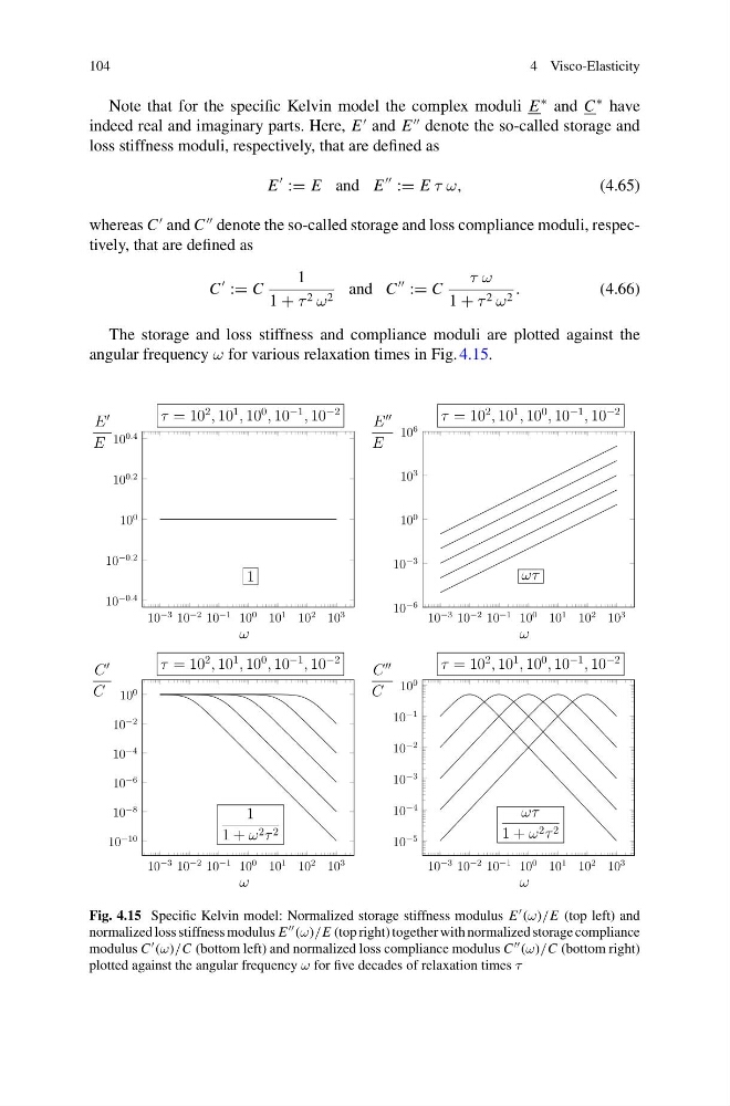
The storage and loss stiffness and compliance moduli are plotted against the
angular frequency ω for various relaxation times in Fig. 4.15.
10
−3 10
−2 10
−1 10
0 10
1 10
2 10
3
10
−0.4
10
−0.2
10
0
10
0.2
10
0.4
ω
E
E
τ = 10
2
, 10
1
, 10
0
, 10
−1
, 10
−2
1
10
−3 10
−2 10
−1 10
0 10
1 10
2 10
3
10
−6
10
−3
10
0
10
3
10
6
ω
E
E
τ = 10
2
, 10
1
, 10
0
, 10
−1
, 10
−2
ωτ
10
−3 10
−2 10
−1 10
0 10
1 10
2 10
3
10
−10
10
−8
10
−6
10
−4
10
−2
10
0
ω
C
C
τ = 10
2
, 10
1
, 10
0
, 10
−1
, 10
−2
1
1 + ω 2 τ 2
10
−3 10
−2 10
−1 10
0 10
1 10
2 10
3
10
−5
10
−4
10
−3
10
−2
10
−1
10
0
ω
C
C
τ = 10
2
, 10
1
, 10
0
, 10
−1
, 10
−2
ωτ
1 + ω 2 τ 2
Fig. 4.15 Specific Kelvin model: Normalized storage stiffness modulus E (ω)/E (top left) and
normalized loss stiffness modulus E (ω)/E (top right) together with normalized storage compliance
modulus C (ω)/C (bottom left) and normalized loss compliance modulus C (ω)/C (bottom right)
plotted against the angular frequency ω for five decades of relaxation times τ
4 Visco-Elasticity
Note that for the specific Kelvin model the complex moduli E
∗ and C
∗ have
indeed real and imaginary parts. Here, E
and E
denote the so-called storage and
loss stiffness moduli, respectively, that are defined as
E
:= E and E
:= E τ ω,
(4.65)
whereas C
and C
denote the so-called storage and loss compliance moduli, respectively, that are defined as
C
:= C
1
1 + τ 2 ω 2 and C
:= C
τ ω
1 + τ 2 ω 2 .
(4.66)
The storage and loss stiffness and compliance moduli are plotted against the
angular frequency ω for various relaxation times in Fig. 4.15.
10
−3 10
−2 10
−1 10
0 10
1 10
2 10
3
10
−0.4
10
−0.2
10
0
10
0.2
10
0.4
ω
E
E
τ = 10
2
, 10
1
, 10
0
, 10
−1
, 10
−2
1
10
−3 10
−2 10
−1 10
0 10
1 10
2 10
3
10
−6
10
−3
10
0
10
3
10
6
ω
E
E
τ = 10
2
, 10
1
, 10
0
, 10
−1
, 10
−2
ωτ
10
−3 10
−2 10
−1 10
0 10
1 10
2 10
3
10
−10
10
−8
10
−6
10
−4
10
−2
10
0
ω
C
C
τ = 10
2
, 10
1
, 10
0
, 10
−1
, 10
−2
1
1 + ω 2 τ 2
10
−3 10
−2 10
−1 10
0 10
1 10
2 10
3
10
−5
10
−4
10
−3
10
−2
10
−1
10
0
ω
C
C
τ = 10
2
, 10
1
, 10
0
, 10
−1
, 10
−2
ωτ
1 + ω 2 τ 2
Fig. 4.15 Specific Kelvin model: Normalized storage stiffness modulus E (ω)/E (top left) and
normalized loss stiffness modulus E (ω)/E (top right) together with normalized storage compliance
modulus C (ω)/C (bottom left) and normalized loss compliance modulus C (ω)/C (bottom right)
plotted against the angular frequency ω for five decades of relaxation times τ