

4.2 Kelvin Model
99
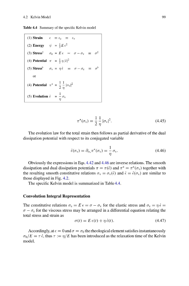
Table 4.4 Summary of the specific Kelvin model
(1) Strain
≡ e ≡ v
(2) Energy ψ =
1
2 E 2
(3) Stress
σ e = E = σ − σ v ≡ σ
(4) Potential π =
1
2 η |˙ | 2
(5) Stress
σ v = η ˙
= σ − σ e ≡ σ
or
(4) Potential π ∗ =
1
2
1
η
|σ v |
2
(5) Evolution ˙
=
1
η
σ v
π
∗
(σ v ) =
1
2
1
η
|σ v |
2
.
(4.45)
The evolution law for the total strain then follows as partial derivative of the dual
dissipation potential with respect to its conjugated variable
˙
(σ v ) = ∂ σ v π
∗
(σ v ) =
1
η
σ v .
(4.46)
Obviously the expressions in Eqs. 4.42 and 4.46 are inverse relations. The smooth
dissipation and dual dissipation potentials π = π(˙ ) and π
∗
= π
∗
(σ v ) together with
the resulting smooth constitutive relations σ v = σ v (˙ ) and ˙
= ˙
(σ v ) are similar to
those displayed in Fig. 4.2.
The specific Kelvin model is summarized in Table 4.4.
Convolution Integral Representation
The constitutive relations σ e = E = σ − σ v for the elastic stress and σ v = η ˙
=
σ − σ e for the viscous stress may be arranged in a differential equation relating the
total stress and strain as
σ(t) = E (t) + η ˙
(t).
(4.47)
Accordingly, at = 0 and σ = σ 0 the rheological element satisfies instantaneously
σ 0 /E = τ ˙
, thus τ := η/E has been introduced as the relaxation time of the Kelvin
model.
99
Table 4.4 Summary of the specific Kelvin model
(1) Strain
≡ e ≡ v
(2) Energy ψ =
1
2 E 2
(3) Stress
σ e = E = σ − σ v ≡ σ
(4) Potential π =
1
2 η |˙ | 2
(5) Stress
σ v = η ˙
= σ − σ e ≡ σ
or
(4) Potential π ∗ =
1
2
1
η
|σ v |
2
(5) Evolution ˙
=
1
η
σ v
π
∗
(σ v ) =
1
2
1
η
|σ v |
2
.
(4.45)
The evolution law for the total strain then follows as partial derivative of the dual
dissipation potential with respect to its conjugated variable
˙
(σ v ) = ∂ σ v π
∗
(σ v ) =
1
η
σ v .
(4.46)
Obviously the expressions in Eqs. 4.42 and 4.46 are inverse relations. The smooth
dissipation and dual dissipation potentials π = π(˙ ) and π
∗
= π
∗
(σ v ) together with
the resulting smooth constitutive relations σ v = σ v (˙ ) and ˙
= ˙
(σ v ) are similar to
those displayed in Fig. 4.2.
The specific Kelvin model is summarized in Table 4.4.
Convolution Integral Representation
The constitutive relations σ e = E = σ − σ v for the elastic stress and σ v = η ˙
=
σ − σ e for the viscous stress may be arranged in a differential equation relating the
total stress and strain as
σ(t) = E (t) + η ˙
(t).
(4.47)
Accordingly, at = 0 and σ = σ 0 the rheological element satisfies instantaneously
σ 0 /E = τ ˙
, thus τ := η/E has been introduced as the relaxation time of the Kelvin
model.