

12
average, this biased variance would not be obvious. In a similar manner, positive and negative SST anomalies might not
be distributed realistically, with the model perhaps producing a few very strong positive anomalies and many weak
negative anomalies that still form the expected average. In
this case, the modeled SST distribution is skewed with
respect to observations.
An additional limitation on the hunt for biases is that a
bias can only be diagnosed in comparison to a reliable observational benchmark. Many parameters of the real climate
system, however, are hard to observe or have only been
observed for a short time. In general, large-scale patterns on
the earth’s surface and throughout the atmosphere can be
observed relatively easily with satellite-borne remote sensing instruments. SST, for example, has been carefully monitored by a number of satellite missions since the 1980s.
Processes below the ocean surface, however, can usually not
be monitored from space. Instead, observational data have to
be obtained by measurements from ships, moored instruments and autonomous vehicles such as gliders and floats.
For the tropical oceans, the TAO/TRITON mooring array in
the Pacific (McPhaden 1995), the PIRATA array in the
Atlantic (Bourlès et al. 2008), and the RAMA array in the
Indian Ocean (McPhaden et al. 2009) provide, among others,
information on temperature, salinity, current velocities and
air-sea fluxes. Additionally, an increasing number of hydrographic observations have become available over the last
decade due to the Argo program (Roemmich et al. 2009).
While all of these measurements provide invaluable information about the state of the tropical oceans, they are not spatially continuous and have only been operational for the last
few decades. Obtaining information about the evolution of
the climate system in the past remains a core challenge of
climate research.
Although no climate model is exactly like the other,
some biases are shared by a wide range of state-of-the-art
CGCMs. Figure 5 shows the global pattern of the annual
mean SST bias for the average of 33 CGCMs and an experiment with the Kiel Climate Model (KCM, Park et al. 2009).
Positive values indicate that modeled SST is warmer than in
observations and vice versa. We validated the performance
of these CGCMs and the KCM in terms of SST against the
satellite derived Optimum Interpolated SST dataset (OISST,
Reynolds et al. 2007; Banzon et al. 2016). Figure 5 shows
that while the KCM is a unique model that has individual
flaws and strengths, the characteristics of its equatorial
Atlantic SST bias are well comparable to other current
CGCMs (examples of other models are shown, among others, in Wahl et al. 2011; Xu et al. 2014; Ding et al. 2015;
Harlaß et al. 2017).
The KCM is a state-of-the-art CGCM that was integrated
with radiative forcing for the period 1981–2012 in rather
coarse resolution. The ocean-sea ice model NEMO (Madec
2008) was run with 31 vertical levels and a horizontal resolution of 2° that is refined to 0.5° in the equatorial region. The
atmospheric model ECHAM5 (Roeckner et al. 2003) is run
with 19 vertical levels and a global horizontal resolution of
approximately 3.75°. Results from KCM simulations are
selected here for consistency reasons. We stress again that
while the KCM differs wildly from other CGCMs in some
aspects, its simulation of the tropical Atlantic is representative for most current-generation CGCMs.
Can Climate Models Reproduce
the Observed Seasonality of the Equatorial
Atlantic Climate System?
The Equatorial Atlantic Warm Bias: Symptoms
The annual mean SST bias varies considerably between
different regions of the ocean (Fig. 5). Striking features of
the global SST bias pattern are the pronounced warm biases
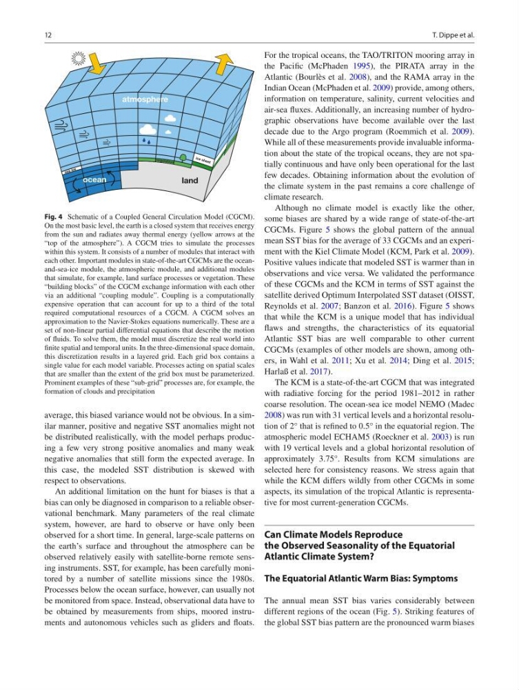
Fig. 4 Schematic of a Coupled General Circulation Model (CGCM).
On the most basic level, the earth is a closed system that receives energy
from the sun and radiates away thermal energy (yellow arrows at the
“top of the atmosphere”). A CGCM tries to simulate the processes
within this system. It consists of a number of modules that interact with
each other. Important modules in state-of-the-art CGCMs are the oceanand- sea-ice module, the atmospheric module, and additional modules
that simulate, for example, land surface processes or vegetation. These
“building blocks” of the CGCM exchange information with each other
via an additional “coupling module”. Coupling is a computationally
expensive operation that can account for up to a third of the total
required computational resources of a CGCM. A CGCM solves an
approximation to the Navier-Stokes equations numerically. These are a
set of non-linear partial differential equations that describe the motion
of fluids. To solve them, the model must discretize the real world into
finite spatial and temporal units. In the three-dimensional space domain,
this discretization results in a layered grid. Each grid box contains a
single value for each model variable. Processes acting on spatial scales
that are smaller than the extent of the grid box must be parameterized.
Prominent examples of these “sub-grid” processes are, for example, the
formation of clouds and precipitation
T. Dippe et al.
average, this biased variance would not be obvious. In a similar manner, positive and negative SST anomalies might not
be distributed realistically, with the model perhaps producing a few very strong positive anomalies and many weak
negative anomalies that still form the expected average. In
this case, the modeled SST distribution is skewed with
respect to observations.
An additional limitation on the hunt for biases is that a
bias can only be diagnosed in comparison to a reliable observational benchmark. Many parameters of the real climate
system, however, are hard to observe or have only been
observed for a short time. In general, large-scale patterns on
the earth’s surface and throughout the atmosphere can be
observed relatively easily with satellite-borne remote sensing instruments. SST, for example, has been carefully monitored by a number of satellite missions since the 1980s.
Processes below the ocean surface, however, can usually not
be monitored from space. Instead, observational data have to
be obtained by measurements from ships, moored instruments and autonomous vehicles such as gliders and floats.
For the tropical oceans, the TAO/TRITON mooring array in
the Pacific (McPhaden 1995), the PIRATA array in the
Atlantic (Bourlès et al. 2008), and the RAMA array in the
Indian Ocean (McPhaden et al. 2009) provide, among others,
information on temperature, salinity, current velocities and
air-sea fluxes. Additionally, an increasing number of hydrographic observations have become available over the last
decade due to the Argo program (Roemmich et al. 2009).
While all of these measurements provide invaluable information about the state of the tropical oceans, they are not spatially continuous and have only been operational for the last
few decades. Obtaining information about the evolution of
the climate system in the past remains a core challenge of
climate research.
Although no climate model is exactly like the other,
some biases are shared by a wide range of state-of-the-art
CGCMs. Figure 5 shows the global pattern of the annual
mean SST bias for the average of 33 CGCMs and an experiment with the Kiel Climate Model (KCM, Park et al. 2009).
Positive values indicate that modeled SST is warmer than in
observations and vice versa. We validated the performance
of these CGCMs and the KCM in terms of SST against the
satellite derived Optimum Interpolated SST dataset (OISST,
Reynolds et al. 2007; Banzon et al. 2016). Figure 5 shows
that while the KCM is a unique model that has individual
flaws and strengths, the characteristics of its equatorial
Atlantic SST bias are well comparable to other current
CGCMs (examples of other models are shown, among others, in Wahl et al. 2011; Xu et al. 2014; Ding et al. 2015;
Harlaß et al. 2017).
The KCM is a state-of-the-art CGCM that was integrated
with radiative forcing for the period 1981–2012 in rather
coarse resolution. The ocean-sea ice model NEMO (Madec
2008) was run with 31 vertical levels and a horizontal resolution of 2° that is refined to 0.5° in the equatorial region. The
atmospheric model ECHAM5 (Roeckner et al. 2003) is run
with 19 vertical levels and a global horizontal resolution of
approximately 3.75°. Results from KCM simulations are
selected here for consistency reasons. We stress again that
while the KCM differs wildly from other CGCMs in some
aspects, its simulation of the tropical Atlantic is representative for most current-generation CGCMs.
Can Climate Models Reproduce
the Observed Seasonality of the Equatorial
Atlantic Climate System?
The Equatorial Atlantic Warm Bias: Symptoms
The annual mean SST bias varies considerably between
different regions of the ocean (Fig. 5). Striking features of
the global SST bias pattern are the pronounced warm biases
Fig. 4 Schematic of a Coupled General Circulation Model (CGCM).
On the most basic level, the earth is a closed system that receives energy
from the sun and radiates away thermal energy (yellow arrows at the
“top of the atmosphere”). A CGCM tries to simulate the processes
within this system. It consists of a number of modules that interact with
each other. Important modules in state-of-the-art CGCMs are the oceanand- sea-ice module, the atmospheric module, and additional modules
that simulate, for example, land surface processes or vegetation. These
“building blocks” of the CGCM exchange information with each other
via an additional “coupling module”. Coupling is a computationally
expensive operation that can account for up to a third of the total
required computational resources of a CGCM. A CGCM solves an
approximation to the Navier-Stokes equations numerically. These are a
set of non-linear partial differential equations that describe the motion
of fluids. To solve them, the model must discretize the real world into
finite spatial and temporal units. In the three-dimensional space domain,
this discretization results in a layered grid. Each grid box contains a
single value for each model variable. Processes acting on spatial scales
that are smaller than the extent of the grid box must be parameterized.
Prominent examples of these “sub-grid” processes are, for example, the
formation of clouds and precipitation
T. Dippe et al.