

6.4 Brownian Dynamics with Hydrodynamic Interactions
87
D ij = D 0 δ ij , i, j on the same particle,
(6.17)
D ij =
3
4
D 0
a
r ij
I +
− → r ij ⊗ − → r ij
r 2
ij
, i, j on different particles
− → r ij ⊗ − → r ij is the dyadic product, for particles i = 1, j = 2, we have
− →
r 12 ⊗ − →
r 12 =
⎡
⎣
x 12
y 12
z 12
⎤
⎦
x 12 y 12 z 12
=
⎡
⎣
x 2
12 x 12 y 12 x 12 z 12
y 12 x 12 y 2
12 y 12 z 12
z 12 x 12 z 12 y 12 z 2
12
⎤
⎦
(6.18)
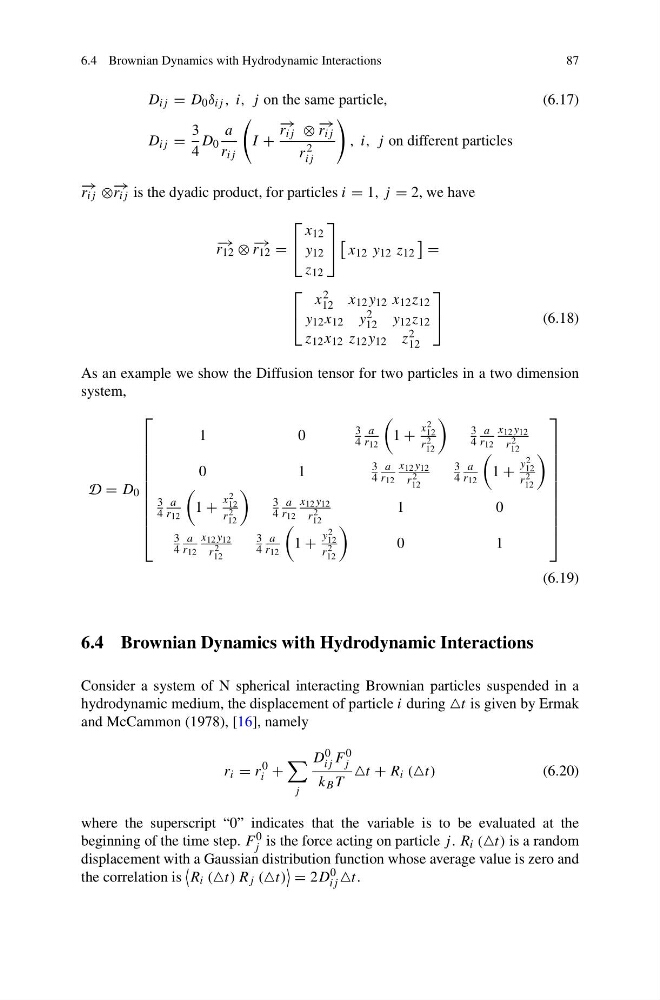
As an example we show the Diffusion tensor for two particles in a two dimension
system,
D = D 0
⎡
⎢
⎢
⎢
⎢
⎢
⎢
⎢
⎢
⎢
⎢
⎣
1
0
3
4
a
r 12
1 +
x 2
12
r 2
12
3
4
a
r 12
x 12 y 12
r 2
12
0
1
3
4
a
r 12
x 12 y 12
r 2
12
3
4
a
r 12
1 +
y 2
12
r 2
12
3
4
a
r 12
1 +
x 2
12
r 2
12
3
4
a
r 12
x 12 y 12
r 2
12
1
0
3
4
a
r 12
x 12 y 12
r 2
12
3
4
a
r 12
1 +
y 2
12
r 2
12
0
1
⎤
⎥
⎥
⎥
⎥
⎥
⎥
⎥
⎥
⎥
⎥
⎦
(6.19)
6.4 Brownian Dynamics with Hydrodynamic Interactions
Consider a system of N spherical interacting Brownian particles suspended in a
hydrodynamic medium, the displacement of particle i during t is given by Ermak
and McCammon (1978), [16], namely
r i = r
0
i +
j
D 0
ij F 0
j
k B T
t + R i (t)
(6.20)
where the superscript “0” indicates that the variable is to be evaluated at the
beginning of the time step. F 0
j is the force acting on particle j . R i (t) is a random
displacement with a Gaussian distribution function whose average value is zero and
the correlation is
R i (t) R j (t)
= 2D 0
ij t.
87
D ij = D 0 δ ij , i, j on the same particle,
(6.17)
D ij =
3
4
D 0
a
r ij
I +
− → r ij ⊗ − → r ij
r 2
ij
, i, j on different particles
− → r ij ⊗ − → r ij is the dyadic product, for particles i = 1, j = 2, we have
− →
r 12 ⊗ − →
r 12 =
⎡
⎣
x 12
y 12
z 12
⎤
⎦
x 12 y 12 z 12
=
⎡
⎣
x 2
12 x 12 y 12 x 12 z 12
y 12 x 12 y 2
12 y 12 z 12
z 12 x 12 z 12 y 12 z 2
12
⎤
⎦
(6.18)
As an example we show the Diffusion tensor for two particles in a two dimension
system,
D = D 0
⎡
⎢
⎢
⎢
⎢
⎢
⎢
⎢
⎢
⎢
⎢
⎣
1
0
3
4
a
r 12
1 +
x 2
12
r 2
12
3
4
a
r 12
x 12 y 12
r 2
12
0
1
3
4
a
r 12
x 12 y 12
r 2
12
3
4
a
r 12
1 +
y 2
12
r 2
12
3
4
a
r 12
1 +
x 2
12
r 2
12
3
4
a
r 12
x 12 y 12
r 2
12
1
0
3
4
a
r 12
x 12 y 12
r 2
12
3
4
a
r 12
1 +
y 2
12
r 2
12
0
1
⎤
⎥
⎥
⎥
⎥
⎥
⎥
⎥
⎥
⎥
⎥
⎦
(6.19)
6.4 Brownian Dynamics with Hydrodynamic Interactions
Consider a system of N spherical interacting Brownian particles suspended in a
hydrodynamic medium, the displacement of particle i during t is given by Ermak
and McCammon (1978), [16], namely
r i = r
0
i +
j
D 0
ij F 0
j
k B T
t + R i (t)
(6.20)
where the superscript “0” indicates that the variable is to be evaluated at the
beginning of the time step. F 0
j is the force acting on particle j . R i (t) is a random
displacement with a Gaussian distribution function whose average value is zero and
the correlation is
R i (t) R j (t)
= 2D 0
ij t.