

72
5 Rotation of a Dipole
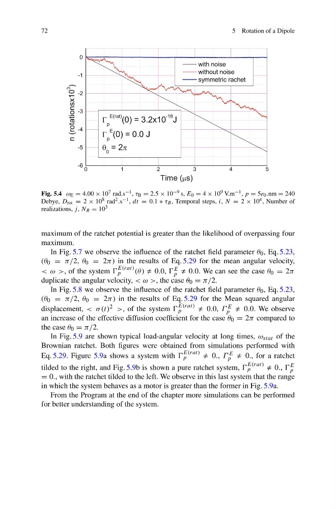
Fig. 5.4 ω E = 4.00 × 10 7 rad.s −1 , τ B = 2.5 × 10 −9 s, E 0 = 4 × 10 9 V.m −1 , p = 5e 0 .nm = 240
Debye, D rot = 2 × 10 8 rad 2 .s −1 , dt = 0.1 ∗ τ B , Temporal steps, i, N = 2 × 10 4 , Number of
realizations, j , N R = 10 3
maximum of the ratchet potential is greater than the likelihood of overpassing four
maximum.
In Fig. 5.7 we observe the influence of the ratchet field parameter θ 0 , Eq. 5.23,
(θ 0 = π/2, θ 0 = 2π ) in the results of Eq. 5.29 for the mean angular velocity,
< ω >, of the system
E(rat)
p
(θ ) 0.0, E
p 0.0. We can see the case θ 0 = 2π
duplicate the angular velocity, < ω >, the case θ 0 = π/2.
In Fig. 5.8 we observe the influence of the ratchet field parameter θ 0 , Eq. 5.23,
(θ 0 = π/2, θ 0 = 2π ) in the results of Eq. 5.29 for the Mean squared angular
displacement, < σ(t) 2 >, of the system
E(rat)
p
0.0, Γ E
p 0.0. We observe
an increase of the effective diffusion coefficient for the case θ 0 = 2π compared to
the case θ 0 = π/2.
In Fig. 5.9 are shown typical load-angular velocity at long times, ω stat of the
Brownian ratchet. Both figures were obtained from simulations performed with
Eq. 5.29. Figure 5.9a shows a system with
E(rat)
p
0., Γ E
p 0., for a ratchet
tilded to the right, and Fig. 5.9b is shown a pure ratchet system,
E(rat)
p
0., E
p
= 0., with the ratchet tilded to the left. We observe in this last system that the range
in which the system behaves as a motor is greater than the former in Fig. 5.9a.
From the Program at the end of the chapter more simulations can be performed
for better understanding of the system.
5 Rotation of a Dipole
Fig. 5.4 ω E = 4.00 × 10 7 rad.s −1 , τ B = 2.5 × 10 −9 s, E 0 = 4 × 10 9 V.m −1 , p = 5e 0 .nm = 240
Debye, D rot = 2 × 10 8 rad 2 .s −1 , dt = 0.1 ∗ τ B , Temporal steps, i, N = 2 × 10 4 , Number of
realizations, j , N R = 10 3
maximum of the ratchet potential is greater than the likelihood of overpassing four
maximum.
In Fig. 5.7 we observe the influence of the ratchet field parameter θ 0 , Eq. 5.23,
(θ 0 = π/2, θ 0 = 2π ) in the results of Eq. 5.29 for the mean angular velocity,
< ω >, of the system
E(rat)
p
(θ ) 0.0, E
p 0.0. We can see the case θ 0 = 2π
duplicate the angular velocity, < ω >, the case θ 0 = π/2.
In Fig. 5.8 we observe the influence of the ratchet field parameter θ 0 , Eq. 5.23,
(θ 0 = π/2, θ 0 = 2π ) in the results of Eq. 5.29 for the Mean squared angular
displacement, < σ(t) 2 >, of the system
E(rat)
p
0.0, Γ E
p 0.0. We observe
an increase of the effective diffusion coefficient for the case θ 0 = 2π compared to
the case θ 0 = π/2.
In Fig. 5.9 are shown typical load-angular velocity at long times, ω stat of the
Brownian ratchet. Both figures were obtained from simulations performed with
Eq. 5.29. Figure 5.9a shows a system with
E(rat)
p
0., Γ E
p 0., for a ratchet
tilded to the right, and Fig. 5.9b is shown a pure ratchet system,
E(rat)
p
0., E
p
= 0., with the ratchet tilded to the left. We observe in this last system that the range
in which the system behaves as a motor is greater than the former in Fig. 5.9a.
From the Program at the end of the chapter more simulations can be performed
for better understanding of the system.