

58
4 The Smoluchowski Model
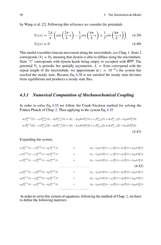
by Wang et al. [2]. Following this reference we consider the potentials:
V 1 (x) =
2A
π
sin
2π
L
x
−
1
2
sin
4π
L
x
+
1
3
sin
6π
L
x
(4.39)
V 2 (x) = 0
(4.40)
This model resembles kinesin movement along the microtubule, see Chap. 1. State 2
corresponds (V 2 = 0), meaning that dynein is able to diffuse along the microtubule.
State “1” corresponds with dynein heads being empty or occupied with ATP. The
potential V 1 is periodic but spatially asymmetric. L = 8 nm correspond with the
repeat length of the microtubule. we approximate at t = 10 −4 s the system has
reached the steady state. Because Eq. 4.38 is not satisfied the steady state deviates
from equilibrium and produces a steady state flux.
4.3.1 Numerical Computation of Mechanochemical Coupling
In order to solve Eq. 4.35 we follow the Crank-Nicolson method for solving the
Fokker-Planck of Chap. 2. Then applying to the system Eq. 4.35
a 1 P
n+1
j
(1) − c 1 P
n+1
j +1 (1) − d 1 P
n+1
j −1 (1) = (b 1 − k 12 dt)P
n
j (1) + c 1 P
n
j +1 (1) + d 1 P
n
j −1 (1) + k 21 dtP
n
j (2)
a 2 P
n+1
j
(2) − c 2 P
n+1
j +1 (2) − d 2 P
n+1
j −1 (2) = (b 2 − k 12 dt)P
n
j (2) + c 2 P
n
j +1 (2) + d 2 P
n
j −1 (2) + k 21 dtP
n
j (2)
(4.41)
Expanding the system,
a 1 P n+1
2
(1) − c 1 P n+1
3
(1) − d 1 P n+1
1
(1)
=
(b 1 − k 12 dt)P n
2 (1) + c 1 P n
3 (1) + d 1 P n
1 (1) + k 21 dtP n
2 (2)
a 1 P n+1
3
(1) − c 1 P n+1
4
(1) − d 1 P n+1
2
(1)
=
(b 1 − k 12 dt)P n
3 (1) + c 1 P n
4 (1) + d 1 P n
2 (1) + k 21 dtP n
3 (2)
a 1 P n+1
4
(1) − c 1 P n+1
5
(1) − d 1 P n+1
3
(1)
=
(b 1 − k 12 dt)P n
4 (1) + c 1 P n
5 (1) + d 1 P n
3 (1) + k 21 dtP n
4 (2)
. . . . . . . . . . . . . . . . . . . . . . . . . . . . . . .
(4.42)
a 2 P n+1
2
(2) − c 2 P n+1
3
(2) − d 2 P n+1
1
(2)
=
(b 2 − k 21 dt)P n
2 (2) + c 2 P n
3 (2) + d 2 P n
1 (2) + k 12 dtP n
2 (1)
a 2 P n+1
3
(2) − c 2 P n+1
4
(2) − d 2 P n+1
2
(2)
=
(b 2 − k 21 dt)P n
3 (2) + c 2 P n
4 (1) + d 2 P n
2 (2) + k 12 dtP n
3 (1)
a 2 P n+1
4
(2) − c 2 P n+1
5
(2) − d 2 P n+1
3
(2)
=
(b 2 − k 21 dt)P n
4 (2) + c 2 P n
5 (2) + d 2 P n
3 (2) + k 12 dtP n
4 (1)
. . . . . . . . . . . . . . . . . . . . . . . . . . . . . . .
In order to solve this system of equations, following the method of Chap. 2, we have
to define the following matrixes:
4 The Smoluchowski Model
by Wang et al. [2]. Following this reference we consider the potentials:
V 1 (x) =
2A
π
sin
2π
L
x
−
1
2
sin
4π
L
x
+
1
3
sin
6π
L
x
(4.39)
V 2 (x) = 0
(4.40)
This model resembles kinesin movement along the microtubule, see Chap. 1. State 2
corresponds (V 2 = 0), meaning that dynein is able to diffuse along the microtubule.
State “1” corresponds with dynein heads being empty or occupied with ATP. The
potential V 1 is periodic but spatially asymmetric. L = 8 nm correspond with the
repeat length of the microtubule. we approximate at t = 10 −4 s the system has
reached the steady state. Because Eq. 4.38 is not satisfied the steady state deviates
from equilibrium and produces a steady state flux.
4.3.1 Numerical Computation of Mechanochemical Coupling
In order to solve Eq. 4.35 we follow the Crank-Nicolson method for solving the
Fokker-Planck of Chap. 2. Then applying to the system Eq. 4.35
a 1 P
n+1
j
(1) − c 1 P
n+1
j +1 (1) − d 1 P
n+1
j −1 (1) = (b 1 − k 12 dt)P
n
j (1) + c 1 P
n
j +1 (1) + d 1 P
n
j −1 (1) + k 21 dtP
n
j (2)
a 2 P
n+1
j
(2) − c 2 P
n+1
j +1 (2) − d 2 P
n+1
j −1 (2) = (b 2 − k 12 dt)P
n
j (2) + c 2 P
n
j +1 (2) + d 2 P
n
j −1 (2) + k 21 dtP
n
j (2)
(4.41)
Expanding the system,
a 1 P n+1
2
(1) − c 1 P n+1
3
(1) − d 1 P n+1
1
(1)
=
(b 1 − k 12 dt)P n
2 (1) + c 1 P n
3 (1) + d 1 P n
1 (1) + k 21 dtP n
2 (2)
a 1 P n+1
3
(1) − c 1 P n+1
4
(1) − d 1 P n+1
2
(1)
=
(b 1 − k 12 dt)P n
3 (1) + c 1 P n
4 (1) + d 1 P n
2 (1) + k 21 dtP n
3 (2)
a 1 P n+1
4
(1) − c 1 P n+1
5
(1) − d 1 P n+1
3
(1)
=
(b 1 − k 12 dt)P n
4 (1) + c 1 P n
5 (1) + d 1 P n
3 (1) + k 21 dtP n
4 (2)
. . . . . . . . . . . . . . . . . . . . . . . . . . . . . . .
(4.42)
a 2 P n+1
2
(2) − c 2 P n+1
3
(2) − d 2 P n+1
1
(2)
=
(b 2 − k 21 dt)P n
2 (2) + c 2 P n
3 (2) + d 2 P n
1 (2) + k 12 dtP n
2 (1)
a 2 P n+1
3
(2) − c 2 P n+1
4
(2) − d 2 P n+1
2
(2)
=
(b 2 − k 21 dt)P n
3 (2) + c 2 P n
4 (1) + d 2 P n
2 (2) + k 12 dtP n
3 (1)
a 2 P n+1
4
(2) − c 2 P n+1
5
(2) − d 2 P n+1
3
(2)
=
(b 2 − k 21 dt)P n
4 (2) + c 2 P n
5 (2) + d 2 P n
3 (2) + k 12 dtP n
4 (1)
. . . . . . . . . . . . . . . . . . . . . . . . . . . . . . .
In order to solve this system of equations, following the method of Chap. 2, we have
to define the following matrixes: