

4.2 Chemical Kinetics
51
J x =
−D
∂C
∂x
Diff usion f lux
−
Drif t velocity
D
k B T
∂V
∂x
C
Drif t f lux
= −D
∂C
∂x
+
∂ (V /k B T )
∂x
C
(4.8)
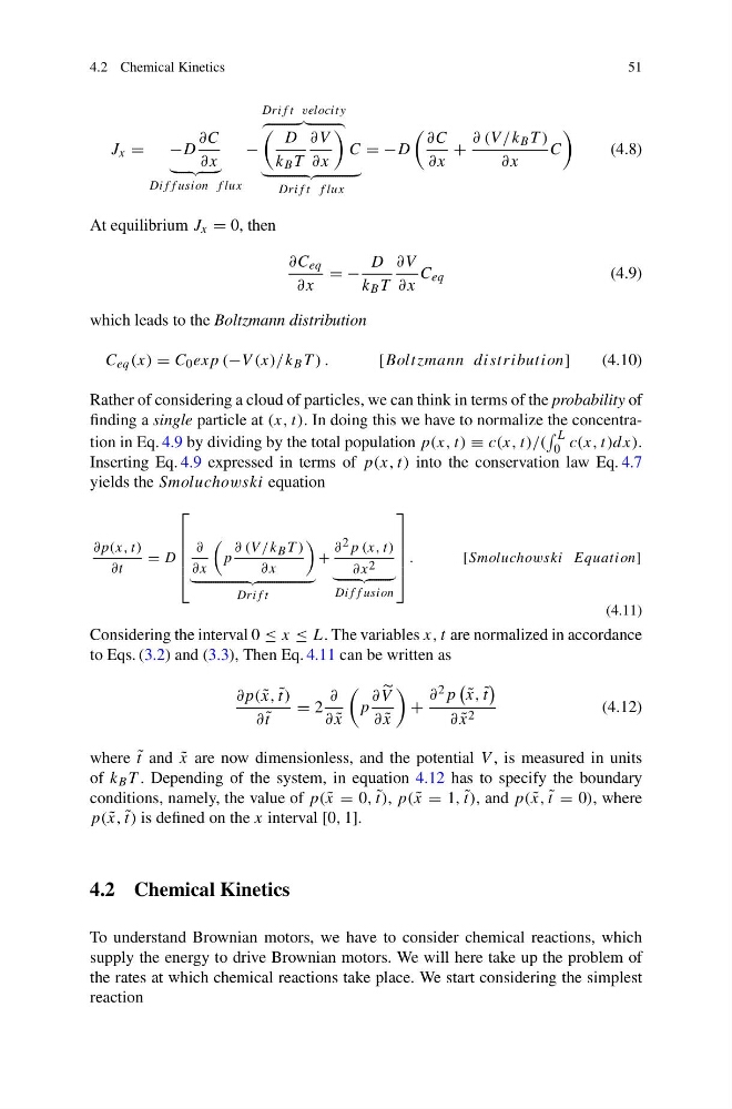
At equilibrium J x = 0, then
∂C eq
∂x
= −
D
k B T
∂V
∂x
C eq
(4.9)
which leads to the Boltzmann distribution
C eq (x) = C 0 exp (−V (x)/k B T ) .
[Boltzmann distribution]
(4.10)
Rather of considering a cloud of particles, we can think in terms of the probability of
finding a single particle at (x, t). In doing this we have to normalize the concentration in Eq. 4.9 by dividing by the total population p(x, t) ≡ c(x, t)/(
L
0 c(x, t)dx).
Inserting Eq. 4.9 expressed in terms of p(x, t) into the conservation law Eq. 4.7
yields the Smoluchowski equation
∂p(x, t)
∂t
= D
⎡
⎢
⎢
⎢
⎢
⎣
∂
∂x
p
∂ (V /k B T )
∂x
Drif t
+
∂ 2 p (x, t)
∂x 2
Diff usion
⎤
⎥
⎥
⎥
⎥
⎦
.
[Smoluchowski Equation]
(4.11)
Considering the interval 0 ≤ x ≤ L. The variables x, t are normalized in accordance
to Eqs. (3.2) and (3.3), Then Eq. 4.11 can be written as
∂p( ˜
x, ˜
t)
∂ ˜
t
= 2
∂
∂ ˜
x
p
∂
V
∂ ˜
x
+
∂ 2 p
˜
x, ˜
t
∂ ˜
x 2
(4.12)
where ˜
t and ˜
x are now dimensionless, and the potential V , is measured in units
of k B T . Depending of the system, in equation 4.12 has to specify the boundary
conditions, namely, the value of p( ˜
x = 0, ˜
t), p( ˜
x = 1, ˜
t), and p( ˜
x, ˜
t = 0), where
p( ˜
x, ˜
t) is defined on the x interval [0, 1].
4.2 Chemical Kinetics
To understand Brownian motors, we have to consider chemical reactions, which
supply the energy to drive Brownian motors. We will here take up the problem of
the rates at which chemical reactions take place. We start considering the simplest
reaction
51
J x =
−D
∂C
∂x
Diff usion f lux
−
Drif t velocity
D
k B T
∂V
∂x
C
Drif t f lux
= −D
∂C
∂x
+
∂ (V /k B T )
∂x
C
(4.8)
At equilibrium J x = 0, then
∂C eq
∂x
= −
D
k B T
∂V
∂x
C eq
(4.9)
which leads to the Boltzmann distribution
C eq (x) = C 0 exp (−V (x)/k B T ) .
[Boltzmann distribution]
(4.10)
Rather of considering a cloud of particles, we can think in terms of the probability of
finding a single particle at (x, t). In doing this we have to normalize the concentration in Eq. 4.9 by dividing by the total population p(x, t) ≡ c(x, t)/(
L
0 c(x, t)dx).
Inserting Eq. 4.9 expressed in terms of p(x, t) into the conservation law Eq. 4.7
yields the Smoluchowski equation
∂p(x, t)
∂t
= D
⎡
⎢
⎢
⎢
⎢
⎣
∂
∂x
p
∂ (V /k B T )
∂x
Drif t
+
∂ 2 p (x, t)
∂x 2
Diff usion
⎤
⎥
⎥
⎥
⎥
⎦
.
[Smoluchowski Equation]
(4.11)
Considering the interval 0 ≤ x ≤ L. The variables x, t are normalized in accordance
to Eqs. (3.2) and (3.3), Then Eq. 4.11 can be written as
∂p( ˜
x, ˜
t)
∂ ˜
t
= 2
∂
∂ ˜
x
p
∂
V
∂ ˜
x
+
∂ 2 p
˜
x, ˜
t
∂ ˜
x 2
(4.12)
where ˜
t and ˜
x are now dimensionless, and the potential V , is measured in units
of k B T . Depending of the system, in equation 4.12 has to specify the boundary
conditions, namely, the value of p( ˜
x = 0, ˜
t), p( ˜
x = 1, ˜
t), and p( ˜
x, ˜
t = 0), where
p( ˜
x, ˜
t) is defined on the x interval [0, 1].
4.2 Chemical Kinetics
To understand Brownian motors, we have to consider chemical reactions, which
supply the energy to drive Brownian motors. We will here take up the problem of
the rates at which chemical reactions take place. We start considering the simplest
reaction