

50
4 The Smoluchowski Model
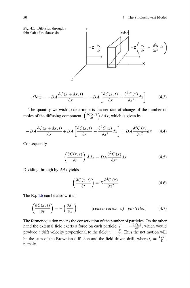
Fig. 4.1 Diffusion through a
thin slab of thickness dx
Z
Y
X
– D
– D
+
∂c
∂x
∂c
∂x
∂
2 c
∂x 2
dx
dx
f low = −DA
∂C(x + dx, t)
∂x
= −DA
∂C(x, t)
∂x
+
∂ 2 C (x)
∂x 2 dx
(4.3)
The quantity we wish to determine is the net rate of change of the number of
moles of the diffusing component.
∂C(x,t)
∂t
Adx, which is given by
−DA
∂C(x + dx, t)
∂x
+DA
∂C(x, t)
∂x
+
∂ 2 C (x)
∂x 2 dx
= DA
∂ 2 C (x)
∂x 2 dx
(4.4)
Consequently
∂C(x, t)
∂t
Adx = DA
∂ 2 C (x)
∂x 2 dx
(4.5)
Dividing through by Adx yields
∂C(x, t)
∂t
= D
∂ 2 C (x)
∂x 2
(4.6)
The Eq. 4.6 can be also written
∂C(x, t)
∂t
= −
∂J x
∂x
.
[conservation of particles]
(4.7)
The former equation means the conservation of the number of particles. On the other
hand the external field exerts a force on each particle, F = −
∂V (x)
∂x , which would
produce a drift velocity proportional to the field: v =
F
ξ . Thus the net motion will
be the sum of the Brownian diffusion and the field-driven drift: where ξ =
k B T
D ,
namely
4 The Smoluchowski Model
Fig. 4.1 Diffusion through a
thin slab of thickness dx
Z
Y
X
– D
– D
+
∂c
∂x
∂c
∂x
∂
2 c
∂x 2
dx
dx
f low = −DA
∂C(x + dx, t)
∂x
= −DA
∂C(x, t)
∂x
+
∂ 2 C (x)
∂x 2 dx
(4.3)
The quantity we wish to determine is the net rate of change of the number of
moles of the diffusing component.
∂C(x,t)
∂t
Adx, which is given by
−DA
∂C(x + dx, t)
∂x
+DA
∂C(x, t)
∂x
+
∂ 2 C (x)
∂x 2 dx
= DA
∂ 2 C (x)
∂x 2 dx
(4.4)
Consequently
∂C(x, t)
∂t
Adx = DA
∂ 2 C (x)
∂x 2 dx
(4.5)
Dividing through by Adx yields
∂C(x, t)
∂t
= D
∂ 2 C (x)
∂x 2
(4.6)
The Eq. 4.6 can be also written
∂C(x, t)
∂t
= −
∂J x
∂x
.
[conservation of particles]
(4.7)
The former equation means the conservation of the number of particles. On the other
hand the external field exerts a force on each particle, F = −
∂V (x)
∂x , which would
produce a drift velocity proportional to the field: v =
F
ξ . Thus the net motion will
be the sum of the Brownian diffusion and the field-driven drift: where ξ =
k B T
D ,
namely