

34
3 Biased Brownian Motion
x n+1 = b or remain at the same site x n = a, we consider the conditional probability
as given by Eq. (3.24), namely,
P (a, t 1 |a, t) =
1
2
1 + e
−2μt
(3.35)
An uniformly distributed random number R between [0, 1] is now generated by
the computer. This number is then compared against the conditional probability
Eq. (3.25). If P (a, t 1 |a, t) > R, then we accept the value of the noise a, i.e., x n = a,
else we accept the value b or x n+1 = b. If the value of noise is b at t 1 (= t +
then we calculate the conditional probability of jumping to another site x n+2 = a at
t 2 (= t 1 + as
P (a, t 2 |b, t 1 ) =
1
2
1 − e
−2μt
(3.36)
On the other hand if the value of the noise is x n+1 = a at t 1 (= t +
we calculate the conditional probability P (a, t 2 |a, t1) using Eq. (3.25). We then
compare P (a, t 2 |b, t1) or P (a, t 2 |a, t 1 ) against another uniformly distributed
random number R 1 between [0, 1].
If P (a, t 2 |b, t1) or P (a, t 2 |a, t1) > R 1 then the value of the noise at t 2 is x n+2 =
a else we accept x n+2 = b. By repeating the procedure we can generate a sequence
of random number η(t) switching between two values a and b. In our case between
−1 and 1. It is important to note that the time interval between the two steps is
always fixed and is equal to t which is much smaller than the correlation time τ c
of the noise ((t τ c ). The Program 3.3 generates the DMN in accordance to the
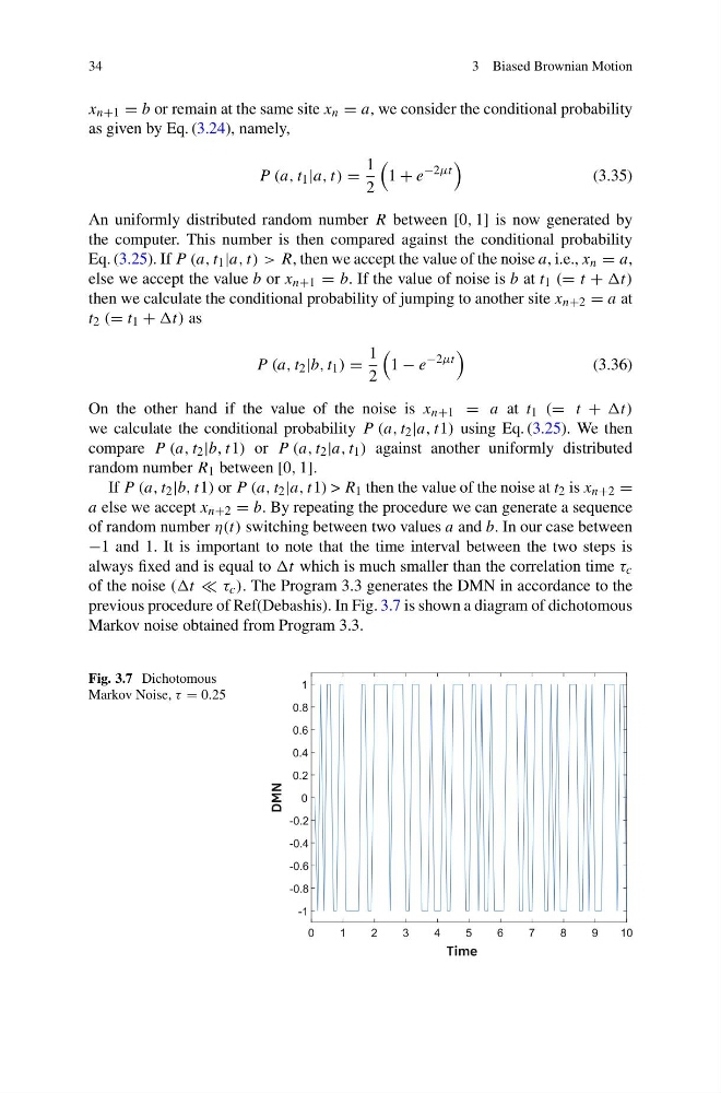
previous procedure of Ref(Debashis). In Fig. 3.7 is shown a diagram of dichotomous
Markov noise obtained from Program 3.3.
Fig. 3.7 Dichotomous
Markov Noise, τ = 0.25
3 Biased Brownian Motion
x n+1 = b or remain at the same site x n = a, we consider the conditional probability
as given by Eq. (3.24), namely,
P (a, t 1 |a, t) =
1
2
1 + e
−2μt
(3.35)
An uniformly distributed random number R between [0, 1] is now generated by
the computer. This number is then compared against the conditional probability
Eq. (3.25). If P (a, t 1 |a, t) > R, then we accept the value of the noise a, i.e., x n = a,
else we accept the value b or x n+1 = b. If the value of noise is b at t 1 (= t +
then we calculate the conditional probability of jumping to another site x n+2 = a at
t 2 (= t 1 + as
P (a, t 2 |b, t 1 ) =
1
2
1 − e
−2μt
(3.36)
On the other hand if the value of the noise is x n+1 = a at t 1 (= t +
we calculate the conditional probability P (a, t 2 |a, t1) using Eq. (3.25). We then
compare P (a, t 2 |b, t1) or P (a, t 2 |a, t 1 ) against another uniformly distributed
random number R 1 between [0, 1].
If P (a, t 2 |b, t1) or P (a, t 2 |a, t1) > R 1 then the value of the noise at t 2 is x n+2 =
a else we accept x n+2 = b. By repeating the procedure we can generate a sequence
of random number η(t) switching between two values a and b. In our case between
−1 and 1. It is important to note that the time interval between the two steps is
always fixed and is equal to t which is much smaller than the correlation time τ c
of the noise ((t τ c ). The Program 3.3 generates the DMN in accordance to the
previous procedure of Ref(Debashis). In Fig. 3.7 is shown a diagram of dichotomous
Markov noise obtained from Program 3.3.
Fig. 3.7 Dichotomous
Markov Noise, τ = 0.25