

3.4 Dichotomous Markov Noise
33
η(t)η(t’) =
D
τ c
exp
−
|t − t’|
τ c
,
(3.32)
where
D = μ b μ a τ c
3 (a + |b|)
2
= μ
2 τ c
3 (2)
2
=
1
2μ
(3.33)
where we have used τ c = (2μ) −1 . Then Eq. (3.18) transforms in,
P =
P (a, t 1 |a, t) P (b, t 1 |a, t)
P (a, t 1 |b, t) P (b, t 1 |b, t)
=
1
2 (1 + e −2μt )
1
2 (1 − e −2μt )
1
2 (1 − e −2μt )
1
2 (1 + e −2μt )
(3.34)
3.4.1 Generating Dichotomous Markov Noise
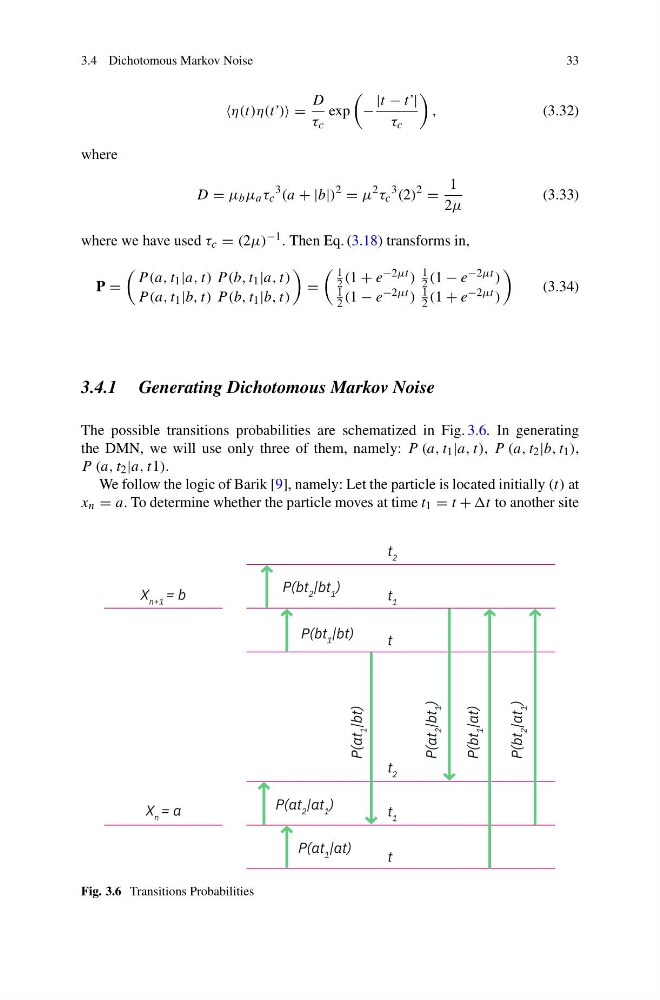
The possible transitions probabilities are schematized in Fig. 3.6. In generating
the DMN, we will use only three of them, namely: P (a, t 1 |a, t), P (a, t 2 |b, t 1 ),
P (a, t 2 |a, t1).
We follow the logic of Barik [9], namely: Let the particle is located initially (t) at
x n = a. To determine whether the particle moves at time t 1 = t + t to another site
Fig. 3.6 Transitions Probabilities
33
η(t)η(t’) =
D
τ c
exp
−
|t − t’|
τ c
,
(3.32)
where
D = μ b μ a τ c
3 (a + |b|)
2
= μ
2 τ c
3 (2)
2
=
1
2μ
(3.33)
where we have used τ c = (2μ) −1 . Then Eq. (3.18) transforms in,
P =
P (a, t 1 |a, t) P (b, t 1 |a, t)
P (a, t 1 |b, t) P (b, t 1 |b, t)
=
1
2 (1 + e −2μt )
1
2 (1 − e −2μt )
1
2 (1 − e −2μt )
1
2 (1 + e −2μt )
(3.34)
3.4.1 Generating Dichotomous Markov Noise
The possible transitions probabilities are schematized in Fig. 3.6. In generating
the DMN, we will use only three of them, namely: P (a, t 1 |a, t), P (a, t 2 |b, t 1 ),
P (a, t 2 |a, t1).
We follow the logic of Barik [9], namely: Let the particle is located initially (t) at
x n = a. To determine whether the particle moves at time t 1 = t + t to another site
Fig. 3.6 Transitions Probabilities