

3.3 Building the Fokker-Plank’s Matrices
27
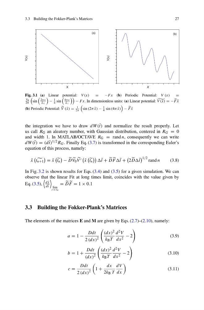
Fig. 3.1 (a) Linear potential: V (x)
=
−F x (b) Periodic Potential: V (x)
=
V 0
2π
sin
2πx
L 1
−
1
4 sin
4πx
L 1
− F x. In dimensionless units: (a) Linear potential:
V ( ˜
x) = −
F ˜
x
(b) Periodic Potential:
V ( ˜
x) =
1
2π
sin (2π ˜
x) −
1
4 sin (4π ˜
x)
−
F ˜
x
the integration we have to draw dW (˜ t) and normalize the result properly. Let
us call R G an aleatory number, with Gaussian distribution, centered in R G = 0
and width 1. In MATLAB/OCTAVE R G = rand n, consequently we can write
dW (˜ t) = (d ˜
t) 1/2 R G . Finally Eq. (3.7) is transformed in the corresponding Euler’s
equation of this process, namely:
˜
x
t n+1
= ˜
x
t n
−
D
V 0
V
˜
x
t n
˜ t +
D
F F˜ t +
2
DD˜ t
1/2 rand n
(3.8)
In Fig. 3.2 is shown results for Eqs. (3.4) and (3.5) for a given simulation. We can
observe that the linear Fit at long times limit, coincides with the value given by
Eq. (3.5),
d ˜
x
d ˜
t
lim
t→∞
=
D
F = 1 × 0.1
3.3 Building the Fokker-Plank’s Matrices
The elements of the matrices E and M are given by Eqs. (2.7)–(2.10), namely:
a = 1 −
Ddt
2 (dx)
2
(dx)
2
k B T
d 2 V
dx 2 − 2
(3.9)
b = 1 +
Ddt
(dx)
2
(dx)
2
k B T
d 2 V
dx 2 − 2
(3.10)
c =
Ddt
2 (dx)
2
1 +
dx
2k B T
dV
dx
(3.11)
27
Fig. 3.1 (a) Linear potential: V (x)
=
−F x (b) Periodic Potential: V (x)
=
V 0
2π
sin
2πx
L 1
−
1
4 sin
4πx
L 1
− F x. In dimensionless units: (a) Linear potential:
V ( ˜
x) = −
F ˜
x
(b) Periodic Potential:
V ( ˜
x) =
1
2π
sin (2π ˜
x) −
1
4 sin (4π ˜
x)
−
F ˜
x
the integration we have to draw dW (˜ t) and normalize the result properly. Let
us call R G an aleatory number, with Gaussian distribution, centered in R G = 0
and width 1. In MATLAB/OCTAVE R G = rand n, consequently we can write
dW (˜ t) = (d ˜
t) 1/2 R G . Finally Eq. (3.7) is transformed in the corresponding Euler’s
equation of this process, namely:
˜
x
t n+1
= ˜
x
t n
−
D
V 0
V
˜
x
t n
˜ t +
D
F F˜ t +
2
DD˜ t
1/2 rand n
(3.8)
In Fig. 3.2 is shown results for Eqs. (3.4) and (3.5) for a given simulation. We can
observe that the linear Fit at long times limit, coincides with the value given by
Eq. (3.5),
d ˜
x
d ˜
t
lim
t→∞
=
D
F = 1 × 0.1
3.3 Building the Fokker-Plank’s Matrices
The elements of the matrices E and M are given by Eqs. (2.7)–(2.10), namely:
a = 1 −
Ddt
2 (dx)
2
(dx)
2
k B T
d 2 V
dx 2 − 2
(3.9)
b = 1 +
Ddt
(dx)
2
(dx)
2
k B T
d 2 V
dx 2 − 2
(3.10)
c =
Ddt
2 (dx)
2
1 +
dx
2k B T
dV
dx
(3.11)