

26
3 Biased Brownian Motion
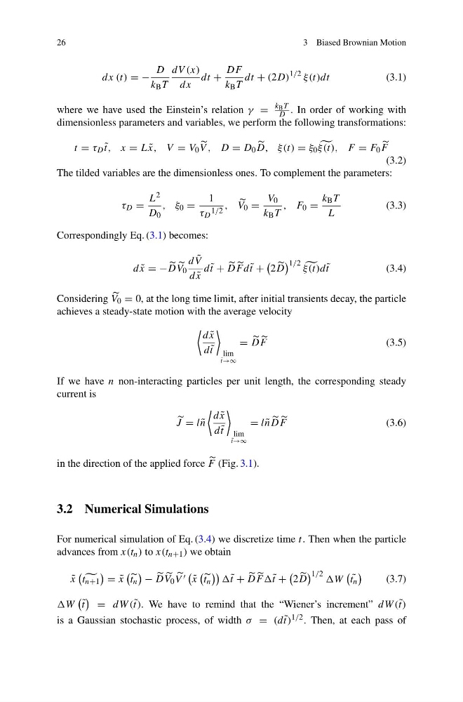
dx (t) = −
D
k B T
dV (x)
dx
dt +
DF
k B T
dt + (2D)
1/2 ξ(t)dt
(3.1)
where we have used the Einstein’s relation γ =
k B T
D . In order of working with
dimensionless parameters and variables, we perform the following transformations:
t = τ D ˜
t, x = L ˜
x, V = V 0
V , D = D 0
D, ξ(t) = ξ 0
ξ(t), F = F 0
F
(3.2)
The tilded variables are the dimensionless ones. To complement the parameters:
τ D =
L 2
D 0
, ξ 0 =
1
τ D
1/2
,
V 0 =
V 0
k B T
, F 0 =
k B T
L
(3.3)
Correspondingly Eq. (3.1) becomes:
d ˜
x = −
D
V 0
d ˜
V
d ˜
x
d ˜
t +
D
F d ˜
t +
2
D
1/2
ξ(t)d ˜
t
(3.4)
Considering
V 0 = 0, at the long time limit, after initial transients decay, the particle
achieves a steady-state motion with the average velocity
d ˜
x
d ˜
t
lim
˜
t→∞
=
D
F
(3.5)
If we have n non-interacting particles per unit length, the corresponding steady
current is
J = l ˜
n
d ˜
x
d ˜
t
lim
˜
t→∞
= l ˜
n
D
F
(3.6)
in the direction of the applied force
F (Fig. 3.1).
3.2 Numerical Simulations
For numerical simulation of Eq. (3.4) we discretize time t. Then when the particle
advances from x(t n ) to x(t n+1 ) we obtain
˜
x
t n+1
= ˜
x
t n
−
D
V 0
V
˜
x
t n
˜ t +
D
F F˜ t +
2
D
1/2 W
˜
t n
(3.7)
W
˜
t
= dW (˜ t). We have to remind that the “Wiener’s increment” dW (˜ t)
is a Gaussian stochastic process, of width σ = (d ˜
t) 1/2 . Then, at each pass of
3 Biased Brownian Motion
dx (t) = −
D
k B T
dV (x)
dx
dt +
DF
k B T
dt + (2D)
1/2 ξ(t)dt
(3.1)
where we have used the Einstein’s relation γ =
k B T
D . In order of working with
dimensionless parameters and variables, we perform the following transformations:
t = τ D ˜
t, x = L ˜
x, V = V 0
V , D = D 0
D, ξ(t) = ξ 0
ξ(t), F = F 0
F
(3.2)
The tilded variables are the dimensionless ones. To complement the parameters:
τ D =
L 2
D 0
, ξ 0 =
1
τ D
1/2
,
V 0 =
V 0
k B T
, F 0 =
k B T
L
(3.3)
Correspondingly Eq. (3.1) becomes:
d ˜
x = −
D
V 0
d ˜
V
d ˜
x
d ˜
t +
D
F d ˜
t +
2
D
1/2
ξ(t)d ˜
t
(3.4)
Considering
V 0 = 0, at the long time limit, after initial transients decay, the particle
achieves a steady-state motion with the average velocity
d ˜
x
d ˜
t
lim
˜
t→∞
=
D
F
(3.5)
If we have n non-interacting particles per unit length, the corresponding steady
current is
J = l ˜
n
d ˜
x
d ˜
t
lim
˜
t→∞
= l ˜
n
D
F
(3.6)
in the direction of the applied force
F (Fig. 3.1).
3.2 Numerical Simulations
For numerical simulation of Eq. (3.4) we discretize time t. Then when the particle
advances from x(t n ) to x(t n+1 ) we obtain
˜
x
t n+1
= ˜
x
t n
−
D
V 0
V
˜
x
t n
˜ t +
D
F F˜ t +
2
D
1/2 W
˜
t n
(3.7)
W
˜
t
= dW (˜ t). We have to remind that the “Wiener’s increment” dW (˜ t)
is a Gaussian stochastic process, of width σ = (d ˜
t) 1/2 . Then, at each pass of